-
Paper Information
- Next Paper
- Previous Paper
- Paper Submission
-
Journal Information
- About This Journal
- Editorial Board
- Current Issue
- Archive
- Author Guidelines
- Contact Us
International Journal of Control Science and Engineering
2012; 2(3): 26-33
doi: 10.5923/j.control.20120203.02
Virtual Metrology Modeling for CVD Film Thickness
 Abstract
 Reference
 Full-Text PDF
 Full-Text HTML
Jérôme Besnard1, Dietmar Gleispach2, Hervé Gris1, Ariane Ferreira3, Agnès Roussy3, Christelle Kernaflen3, Günter Hayderer2
1PDF Solutions, Montpellier, France
2austriamicrosystems AG Unterpremstätten, Austria
3Department of Manufacturing Science and Logistics Ecole Nationale Supérieure des Mines de Saint-Etienne Gardanne, France
Correspondence to: Dietmar Gleispach, austriamicrosystems AG Unterpremstätten, Austria.
| Email: |  |
Copyright © 2012 Scientific & Academic Publishing. All Rights Reserved.
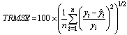
The semiconductor industry is continuously facing four main challenges in film characterization techniques: accuracy, speed, throughput and flexibility. Virtual Metrology (VM), defined as the prediction of metrology variables using process and wafer state information, is able to successfully address these four challenges. VM is understood as definition and application of predictive and corrective mathematical models to specify metrology outputs (physical measurements). These statistical models are based on metrology data and equipment parameters. The objective of this study is to develop a model predicting the CVD oxide thickness (average) for an IMD (Inter Metal Dielectric) deposition process using FDC data (Fault Detection and Classification) and metrology data. In this paper, two VM models are studied: one based on Partial Least Squares Regression (PLS) and one based on Tree ensembles. We will demonstrate that both models show good predictive strength. Finally, we will highlight that model update is key for ensuring a good model robustness over time and that an indicator of confidence of the predicted values is necessary too if the VM model has to be use on-line in a production environment.
Keywords: Advanced Process Control, CVD Oxide Thickness, Partial Least Squares Regression, Tree Ensembles, Semiconductor Manufacturing, Virtual Metrology, Model Update, Indicator of Confidence
Article Outline
1. Introduction
- The semiconductor manufacturing industry has a large- volume multistage manufacturing system. To ensure high stability and high production yield, reliable and accurate process monitoring is required[1]. Advanced Process Control (APC) is currently deployed for factory-wide control of wafer processing in semiconductor manufacturing. The APC tools are considered to be the main drivers to guarantee a continuous process improvement[2]. However, most APC tools strongly depend on the physical measurement provided by metrology tools[3]. Critical wafer parameters are measured, such as, for example, the thickness and/or the uniformity of thin films. If a wafer is misprocessed in an early stage but detected at the wafer acceptance test, unnecessary resource consumption is unavoidable. Measuring every wafer’s quality after each process step could avoid late wafer scraps but it is too expensive and time consuming. Therefore, metrology, as it is employed for product quality monitoring today, can only cover a small fraction of sampled wafers. Virtual metrology (VM) in contrast enables prediction of every wafer’s metrology measurement based on production equipment data and previous metrology results[4-7, 27]. This is achieved by defining and applying predictive models for metrology outputs (physical measurements) as a function of metrology and equipment data of current and previous steps of fabrication[8-10,28-31].Of course it is necessary to collect data from equipment sensors to characterize physical and chemical reactions in the process chamber. Sensor data will constitute the basis for the statistical models that will be developed. A typical Fault Detection and Classification (FDC) system collects on-line sensor data from the processing equipment by sensors for every wafer or batch. They are called process variables or FDC data. Reliable and accurate FDC data are essential in VM model [11]. The objective of a VM module is to develop a robust prediction that can provide estimation of metrology and which is able to handle process drifts whether they are induced by preventive maintenance actions or not.This paper deals with the prediction of PECVD (Plasma Enhanced Chemical Vapor Deposition) oxide thickness for an Inter Metal Dielectric (IMD) layers using FDC and metrology data. Two types of mathematical models are studied to build VM modules for PECVD processes. Partial Least Squares Regression (PLS)[12-13] and a non-linear approach based on Tree ensembles[14-16] are considered. The technical challenge and innovation are to build a single robust model, either with PLS or Tree ensembles, which is valid for several products, different layers and two different chucks. The alternative would be to make a model per layer, chuck and product, but we strongly believe that the maintenance of many single models, in our case 12 different models, is not compatible with the constraints of the industry.Section II deals with fabrication process. In section III we present the mathematical background to build VM models. Results are described in sections IV. Some perspectives about what the next steps of this work will be are given in section V. Finally, section V concludes this paper with a summary.
1.1. Fabrication Process
- The film layer under investigation for thickness modeling is part of the IMD used in the Back-End of Line (BEOL) of a 0.35µm technology process. This oxide layer is used three times during the production of a four metal layer device. PECVD USG (Undoped Silicon Glass) films are commonly used to fill the gaps between metal lines due to their conformal step coverage characteristics. However, as the device geometry is shrinking, the gap fill capability of USG films is no longer sufficient. State of the art technique is the combination of HDP (High Density Plasma) and USG films to provide a high-productivity and low-cost solution. HDP is used to fill the gap just enough to cover the top of the metal line and then the USG is used as a cap layer on top of the HDP oxide film[17].
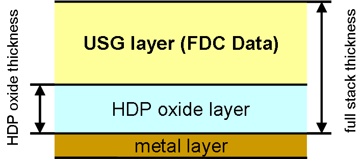 | Figure 1. Layer structure for inter metal dielectric |
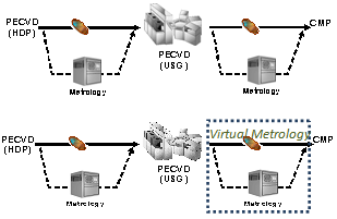 | Figure 2. Process flow |
2. Mathematical Models
2.1. Notation
- The following notation conventions are used in this paper: scalars are designated using lowercase italics. Vectors are generally interpreted as column vectors and are designated using bold italic lowercase (i.e. x). Matrices are shown in bold italic uppercase (i.e. X), where xij, with (i=1,…, I) and (j=1,…, J), is the ijth element of X(I×J). Let X of
 be an input data set and Y of
  be arranged in the following way:
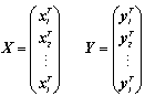 where
where  and
and  . The characters I, J, N, p, q, m and n are reserved for indicating the dimension of vectors and matrices of data.
2.2. VM Modeling
- There are some important points when designing the mathematical models and a methodology that should be considered. In this section we propose two successive stages to deploy mathematical models in order to build a VM Module for an individual process:
2.2.1. Data partitioning: Training set and Test Set
- Let X (I×p) and Y (I×m) be the available data set (cleaned and normalized) respectively from production and metrology process. The data set partitioning consist in the extraction of two units: a unit of 70% of the data set for the training-validation (training and cross validation) and a unit of 30% of the data set for the test. Let XN (N×p) and YN (N×m) be the training-validation data set, and let XN (n×p) and YN (n×m) be the test data set with N+n=I. It is possible to split the available data set in a temporal way (chronological selection) without loss of representativeness. In this case study we have chosen this type of data partitioning before the application of the three mathematical models.Alternatively, the Kennard-Stone method [15] can be used to perform the data set partitioning. The inputs variables domain X of
 ,
,  is considered for the Kennard-Stone method.. It is a sequential method to select a training set uniformly which covers the entire X variable’s space. The selection criteria use the Euclidean distance.
 2.2.2. Mathematical Modeling
- A linear regression model of a given process can be written as:
 | (1) |
 | (2) |
 | (3) |
2.3. PLS Models
- Consider a set of historical process data consisting of an (I × p) matrix of process variable measurements (FDC data) X and a corresponding (I × m) matrix of metrology data Y. Projection to Latent Structures or Partial Least Squares (PLS) can be applied to the matrices X and Y to estimate the coefficient matrix B in (1).
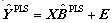 | (4) |
 is the PLS estimate of the process output Y. PLS modeling consists of simultaneous projections of both the X and Y spaces on low dimensional hyper planes of the latent components. This is achieved by simultaneously reducing the dimensions of X and Y, by seeking q (< p) latent variables which mainly explains covariance between X and Y. Therefore this method is useful to obtain a group of latent variables which explain the variability of both, Y and X. The latent variable models for linear spaces are given by Equations (5) and (6) [12]:
 | (5) |
 | (6) |
 | (7) |
 | (8) |
 | (9) |
 | (10) |
2.4. Tree Ensemble Models
- It has been shown by Breiman et al.[22], in the classification case, that under reasonable assumptions, an ensemble procedure allows getting accurate models. Indeed, if the base model has a low-bias and high variance under some random perturbation of the learning conditions, then aggregating a large family of such models give birth to a low-bias, low variance aggregated model, that is more accurate than the individuals models[15].To allow such results to hold, it is critical that the individual models are as independently built as possible, while maintaining low bias. Tree base learners, either based on algorithms such as CART[22] or C4.5[23], are known to have a low bias when fully learned (no pruning)[24]. In order to be able to build families of trees that have a low correlation to one another, from a finite dataset, several methods have been proposed: Bootstrapping the learning set (also known as bagging methods), Random splits, Injecting random noise in the response or building random artificial features as (linear) combinations of the existing ones. All these ideas aim at learning trees that are as uncorrelated as possible.Following Breiman[22], we use here a combination of bagging from the base learning set, and random splits as our main ensemble method. Base learners are regression trees, following a modified CART algorithm for tree learning. Given X, a set of (I × p) FDC data, and a corresponding Y (I × m) metrology, and 2 parameters q (random selection among features at the individual split level) and nTrees (number of trees grown and aggregated), the algorithm is as follows:1. Iterating over the m responses:2. Looping 1 -> nTrees:a) Build a bootstrap sample (I × p) Xb and corresponding Yb (I × 1) responseb) Build a fully-grown tree τ, following modified CART algorithmi. randomly selecting q
3. Results
- In this section we present the results of two different models (PLS and tree ensembles) for prediction of the PECVD oxide film thickness.
3.1. PLS Models with 3 Qualitative Variables
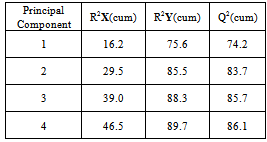
- A PLS model is built without input variable selection. The model is calibrated with 306 wafers of the training validation data set. The 168 wafers of the test data set are used to validate the model. The input variables of the PLS model are the 24 quantitative FDC indicators and the three qualitative variables which are chuck, layer and product. The PLS model with four principal components is selected by cross-validation. Q2(cum) is increasing for the first four principal components and decreasing for the fifth principal component. Actually, using the first four principal components, 46.5% of the X variability (quantitative and qualitative variables) can explain 89.7% of the output Y (average thickness) variability (see table I). Therefore the best statistical model is achieved by using only four principal components.
|
|
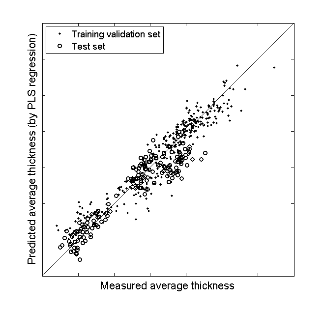 | Figure 3. Predicted average thickness (by PLS model) versus measured average thickness representation |
3.2. Tree Ensembles Model
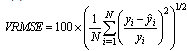
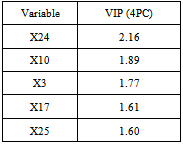
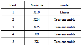
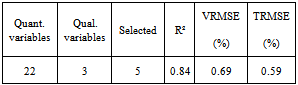
- Modeling is done using the learning set of 306 wafers. After one iteration of the algorithm, one indicator (X10) is selected for the prelinear part; the remaining 26 are left for tree ensemble modeling, including the three qualitative parameters chuck, product and layer. The second iteration of the algorithm provides a model that selected five parameters: X10 in the linear part of the model, and four in the tree ensemble model (X9, X8, X24 and X25). X24 and 25 are two qualitative parameters (see table III). R2 is estimated to be 0.84, being defined as equation (13).
|
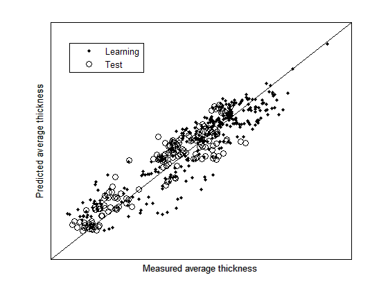 | Figure 4. Predicted average thickness (by tree ensemble model) versus measured average thickness representation |
|
4. Perspectives
- In this paper we have been comparing two different types of mathematical modeling (PLS vs. Tree Ensembles). This academic study can be considered as the first step for virtual metrology, and demonstrates that here, with reasonable parameter selection; different algorithms yield similar results in terms of prediction capacity. So modeling capacity will contribute a low part to the algorithmic choices to be made in virtual metrology, we think. However, two main challenges remain to be addressed before using online virtual metrology prediction in Fab environment. The first one is to ensure VM models will be robust enough with time; this has to deal with model update approaches. The second one is to guarantee that predicted values can be trustfully used; this will be addressed by developing an indicator of confidence for each predicted value. The ultimate goal is to provide a reliable prediction that can be used for the CMP step.The model robustness over time is a key topic that must not be neglected. Many factors can impact the model validity such as the chamber aging, a sudden chamber malfunction, as well as the unscheduled and scheduled preventive maintenances [25]. All these events might lead to a change with time of some collected variables, used as model input on the form of FDC indicators. It is difficult assessing ahead the impact that such changes might have on the model validity. For all these reasons, a static model, built on a leaning dataset with no further updates, doesn’t seem to be a sustainable solution. One should prefer an approach based on dynamic models. In that case, many possibilities exist such as a regular update, a data-driven update (based on estimated quality of the model) and a chamber-driven update (based on maintenance events).
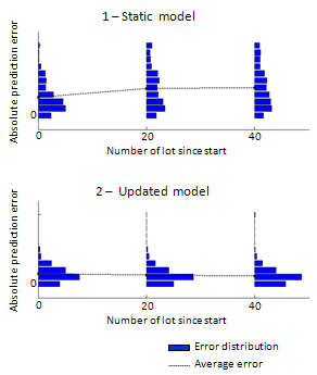 | Figure 5. Comparing the evolution of errors distribution between updating and non-updating models |
5. Conclusions
- This paper presents two mathematical models that have been used to develop virtual metrology for predicting the average oxide film thickness deposited during a PECVD process. The two models have good predictive strength. PLS and tree ensemble show equivalent performance on the test set, but PLS shows slightly better results on the learning set. This could be explained by the elimination of an outlier value (point with highest measure thickness) in learning set of PLS model. PLS uses four principal components, which are based on all the variables. The tree ensemble model uses five variables only. Three out of the top five most important variables of PLS are used in the tree ensemble model.The predictive results are in excellent agreement with the measured data. In addition, we have shown as a novelty in virtual metrology that it is possible to create a single model for different layer, different products and for one chamber with two different chucks. The first results we have had on model update techniques, as well as on building a predictive quality index are very encouraging to reach our final goal which is to have Virtual Metrology running online in the CMP step.
ACKNOWLEDGMENTS
- This work was supported by ENIAC project IMPROVE (Implementing Manufacturing science solutions to increase equipment pROductiVity and fab pErformance). Funding by the EU, the FFG and the MINEFI is gratefully acknowledged.