1. Introduction

The fundamentals of vector control implementation can be explained with the help of Figure 1, where the machine model is presented in a synchronous rotating reference frame. The inverter is omitted from the figure, assuming that it has unity current gain, that is, it generates currents , , and as dictated by the corresponding command currents , , and from the controller. A machine model with internal conversions is shown on the right. The machine terminal phase currents , , and are converted to and components by transformation. These are then converted to synchronously rotating frame by the unit vector components and before applying them to the machine model. The controller makes two stages of inverse transformation, as shown, so that the control currents and correspond to the machine currents and , respectively.

In addition, the unit vector assures correct alignment ofwith the and perpendicular to it, as shown.The transformation and inverse transformation including the inverter ideally do not incorporate any dynamics and therefore, the response to and is instantaneous (neglecting computational and sampling delays).

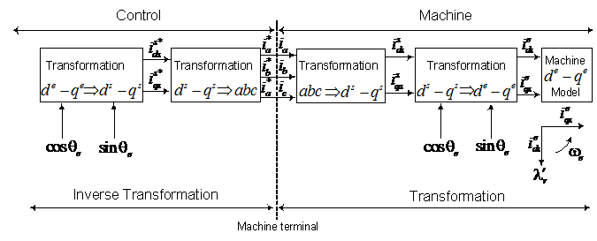Figure 1. Vector control implementation principle with machine dq model

There are two essentially general methods of vector control; one called the direct method, and the other known as the indirect method. The methods are different essentially by how the unit vector (and ) is generated for the control. It should be mentioned that the orientation of with the rotor flux , air gap flux, or stator flux is possible in vector control. However, rotor flux orientation gives natural decoupling control, whereas air gap or stator flux orientation gives a coupling effect which has to be compensated by a decoupling compensation current [1,2].

2. Indirect Field Oriented Control

Indirect vector control is very popular in industrial applications. Figure 2 explains the fundamental principle of indirect vector control with the help of a phasor diagram. The axes are fixed on the stator, but the axes, which are fixed on the rotor, are moving at speed . Synchronously rotating axes are rotating ahead of the axes by the positive slip angle corresponding to slip frequency . Since the rotor pole is directed on the axis and , one can write

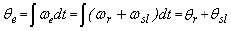(1)

Figure 2. Phasor diagram explaining indirect vector control

The phasor diagram suggests that for decoupling control, the stator flux component of current should be aligned on the axis, and the torque component of current should be on the axis, as shown.

For decoupling control, one can make a derivation of control equations of indirect vector control with the help of dynamic model of induction machine (IM) [1,2,3,4],

(2)

(3)

If-axis is aligned with the rotor field, the q-component of the rotor field, , in the chosen reference frame would be zero [1,2,5,6],

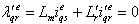(4)

(5)

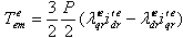
With zero, the equation of the developed torque, Eq.(3), reduces to

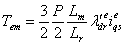(6)

Which shows that if the rotor flux linkage is not disturbed, the torque can be independently controlled by adjusting the stator q component current, .

For to remain unchanged at zero, its time derivative () must be zero, one can show from Eq.(2) [6,1,2]

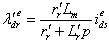(7)

(8)

To implement the indirect vector control strategy, it is necessary to use the condition in Eq.s(6), (7), and (8) in order to satisfy the condition for proper orientation. Torque can be controlled by regulating and slip speed . Given some desired level of rotor flux, , the desired value of may be obtained from,

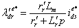(9)

For the desired torque of at the given level of rotor flux, the desired value of in accordance with Eq.(6) is

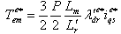(10)

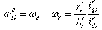
When the field is properly oriented, is zero, : thus, the slip speed of Eq.(8) can be written as

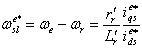(11)

Thus, the above analysis shows that the vector control strategy can provide the same performance as is achieved from a separately excited DC machine; this is done by formulating the stator current phasor, in the two-axis synchronously rotating reference frame, to have two components: magnetizing current component and torque producing current component. The generated motor torque is the product of two. By keeping the magnetizing current component at a constant rated value, the motor torque is linearly proportional to the torque-producing component, which is quite similar to the control of a separately excited DC motor [7,8,9].

3. Indirect Field Orientation Detuning

The success of FOC is based on the proper division of stator current into two components. Using the above d-q axis orientation approach, these two currents components are and , which specify the magnetizing flux and torque respectively [1,2,4,10].

The indirect FOC method uses a feedforward slip calculation to partition the stator current. The slip speed equation is rearranged as

(12)

Where . The above condition, if satisfied, ensures the decoupling torque and flux production; a change in will not disturb the flux and the instantaneous torque control is achieved. This indicates that an ideal field orientation occurs. To what extent this decoupling is actually achieved will depend on the accuracy of motor parameters used. It is easy to be noted that the calculation of the slip frequency in Eq.(12) depends on the rotor resistance. Owing to saturation and heating, the rotor resistance changes and hence the slip frequency is either over or under estimated. Eventually, the rotor flux and the stator-axis current will be no longer decoupled in Eq.(10) and the instantaneous torque control is lost. Furthermore, the electromechanical torque generation is reduced at steady state under the plant parameter variations and hence the machine will work in a low-efficiency region. Finally, the variation of the parameters of moment of inertia J and the friction constant B is common in real applications. For instance, the bearing friction will change after the motor has run for a period of time [11].

Since the values of rotor resistance and magnetizing inductance are known to vary somewhat more than the other parameters, on-line parameter adaptive techniques are often employed to tune the value of these parameters used in an indirect field-oriented controller to ensure proper operation [2,11,12]. The detuning effect, generally, causes degradation in the drive performance.

4. Simulation Results

4.1. Simulation of Fixed Voltage Open-Loop Operation

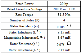
The model equations of the IM, Eq.(2), in the stationary qd reference frame are modeled using SIMULINK [13,14]. The simulation is set up for simulating the dynamic behavior of the motor with fixed-step type. The results from these open-loop operations will later be used as a benchmark to compare the performance of the same motor operated with field-oriented control.

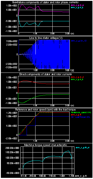
In the model, three-phase voltages of base frequency (=50 Hz) applied to the input are converted into two-phase stationary reference frame voltages. Once d-q phase voltages obtained, the associated flux and current are calculated and then applied to electromechanical and mechanical torque equations to obtain torque-speed responses.

One can see from Figure 3 the monotonic response of the magnetization current before it reaches its steady-sate value (about 82A) and how well the flux amplitude remains constant when the load torque is not constant.

The value of the externally applied mechanical torque is generated by a repeating sequence source with the time and output values scheduled as shown in Figure 3.

Sample results show that the electromechanical torque response of Figure 3 is smooth in case of IFOC, while it is oscillatory in open loop case shown in [1].

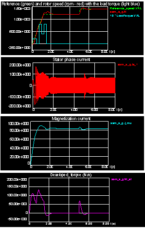Figure 3. Startup and load transients with field-oriented control

4.2. Simulation of IFOC developed in Stationary Reference Frame and Frequency Converter

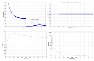
This simulation is implemented to be familiar with indirect field-oriented control and to observe the variables at every stage of the control.

The validity of IFOC technique is verified via two tests. In the first test, a change in stator quadrature current is generated by applying a variable value of the main inductance of the motor as shown in Figure 4a or as shown in Figure 4b by applying a repeating sequence source with the time and output values scheduled as follows:

time_change_iqse= [ 0 0.6 0.8 0.9 2]

output_change_iqse= [0 0 10 10 0 0]

Figure 4a. Changes in Responses due to a change in the magnetization current

Figure 4b. Changes in Responses due to a change in quadrature current

And added to the commanded quadrature stator current in synchronous frame . The same change values are fed to the direct stator current in synchronous frame in the other test. The reflection of these changes on the output synchronous qd components of the stator currents, and , and then to what extent the IFOC technique performs the decoupling action is investigated in Figures 4 and 5.

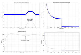Figure 5. Changes in Responses due to change in

In Figure 4, the change in immediately appears at its corresponding output, , while no change is detected in and rotor flux magnitude . Also, the figure shows the change in the response of developed torque and rotor speed due to this current change

In Figure 5, the change in gives rise to a corresponding change in , which in turn affects the response of rotor flux magnitude . No reflection of this change to has been seen, and therefore, no change in the torque and speed responses would be expected.

Thus, the observations seen in Figures 4 and 5 give a strong indication that the decoupling action is well performed by IFOC technique and the machine is, by now, a dc like machine. However, the conclusion that induction machine model has been converted to dc like machine is not yet decisive. There is still a problem behind the calculation of slip frequency, where the changes in rotor resistance could cause degradation in IFOC technique performance and the coupling effect might again be arisen.

4.3. Simulation of IFOC IM with Detuning Effect:

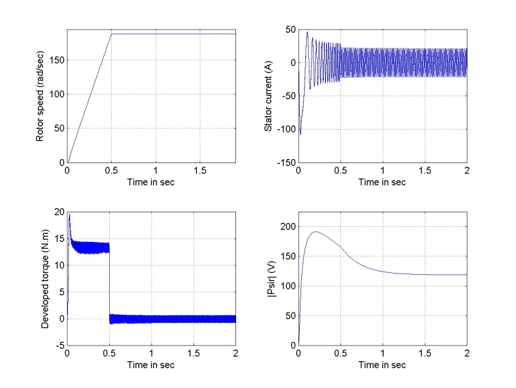
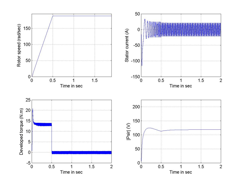
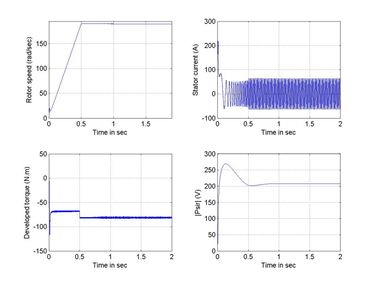
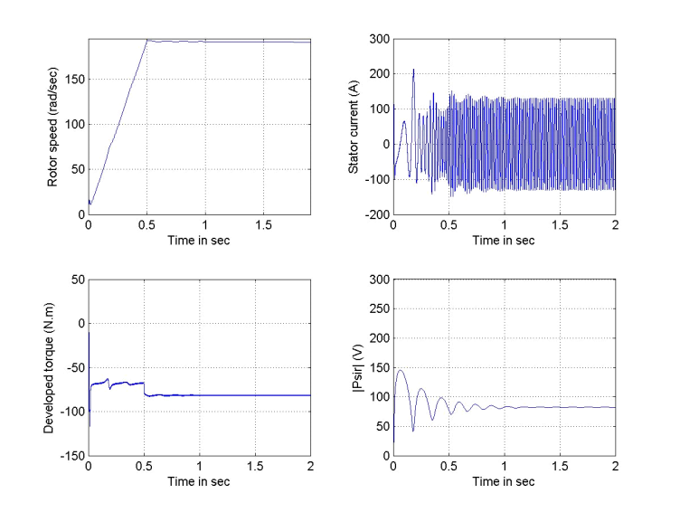
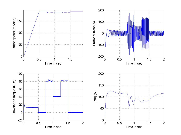
The examination of detuning effect in the rotor resistance is performed by introducing an estimation factor, , to all the terms of machine model. As set up, perfect tuning is when =1. The previous run of perfect tuning, Figure 3, is repeated at fixed reference speed (ramped up to speed in 0.5 sec) for a =1.5 and 0.5, with no-load, rated load and with cyclic change of load.

Figures 6 and 7 are run with no-load and with estimation factors kr=0.5 and 1.5 respectively. It is evident from these figures that the speed responses are not much affected by this change in rotor resistance, where both responses reaches settling time at 0.5 sec. However, their steady state values never reaches the value of the reference value as in the case where kr=1. But, the dramatic changes are observed in the flux linkage levels and their time constants. The level of flux linkage in Figure 6 is higher than that in Figure 7, but the response time of Figure 6 is slower than for Figure 7; a valid justification, since the flux linkage time constant is inversely proportional to the rotor resistance value.

The above run is repeated with rated load torque (Trated=81.49), and the responses of Figure 8 and Figure 9 will be obtained. The speed responses obtained from this test show a temporary jump at motor start-up. Moreover, the steady state speed errors resulting from this test are larger than that with no-load test; with kr=0.5, the speed settles at 189.64 rad/s , while it settles at 191 rad/s when kr=1.5. It is clear from the figures that the developed torque response with kr=1.5 is much distorted as compared to the smooth envelope in case kr=0.5. Also, the current waveform shows a larger swing when kr=1.5 as compared to waveform with kr=0.5. Finally, Figure 10 shows an oscillatory and low level flux linkage compared to the monotonic and higher level flux response in Figure 9, with kr=0.5.

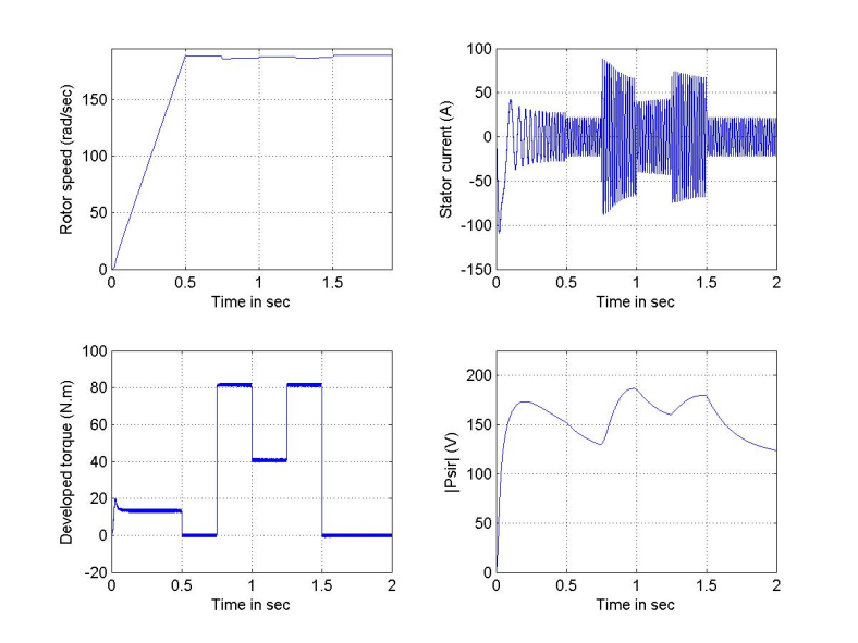
In the next study, the machine is subjected to the same sequence of step changes in load torque as previously applied in perfect tuning, Figure 4. As compared to the perfect tuning case, the increased value of rotor resistance (1.5) could cause the responses of flux linkages, torque and current to be distorted, especially, at time of load exertion, as shown in Figure 10. Also, at this time the speed deviation from its steady state value is larger than the case with kr=1. The situation with the decreased rotor resistance is shown in Figure 11. The responses of Figure 11 are run with kr=0.625; the minimum allowable value below which fluctuations will appear at the developed toque response at load exertion times. One can easily observe the amount of deviation in rotor flux linkage, speed and current responses as compared to the perfect tuning case.

Table 1. Induction Motor Parameter

Figure 6. Responses due to detuning effect (kr=0.5) with no-load

Figure 7. Responses due to detuning effect (kr=1.5) with no-load

Figure 8. Responses due to detuning effect (kr=0.5) with rated load torque

Figure 9. Responses due to detuning effect (kr=1.5) with rated load torque

Figure 10. Responses due to detuning effect (kr=1.5) with cyclic load changes

Figure 11. Responses due to detuning effect (kr=0.625) with cyclic load changes

5. Conclusions

The implementation of IFOC technique has been performed and the following observations could be concluded:

1. he technique can keep the rotor flux constant even during changes in load torque. This indicates that decoupling control of flux and torque has been obtained.

2. It has been shown that decoupling is conditioned by the accuracy of slip calculation. The slip calculation depends on the rotor time constant, , which varies continuously according to the operational conditions.

3. On the other hand, the conventional PI controller can not compensate such parameter variations in the plant. That is, the PI controller is not an intelligent controller nor is the slip calculation accurate. Therefore, changes in degrade the speed performance and other controllers can been suggested.

ACKNOWLEDGEMENTS

Rami A. Maher received the M.S. and Ph.D. degrees in technical cybernetics in 1982 and 1986 from VAAZ -Brno-Czechoslovakia. Since 2007 he has been with Isra-University-Jordan. His main research interests include automatic control theory, and controller design for electromechanical systems, RamiAmahir@yahoo.com.

Walid Emar received the M.Sc. degree in industrial electronics and the Ph.D. degree in automatic control from West Bohemia University, Czech Republic. Currently, He is now teaching at Al-Isra Private University in Jordan as a full-time assistant professor. He is engaged in research of high power multilevel converters for industrial and traction applications, as well as dc/dc regulators,WalidEmar@yahoo.com.