Hanzel Lárez , Hugo Leiva , Darwin Mendoza
Departamento de Matemática, Universidad de Los Andes, Mérida, 5101, Venezuela
Correspondence to: Hugo Leiva , Departamento de Matemática, Universidad de Los Andes, Mérida, 5101, Venezuela.
| Email: |  |
Copyright © 2012 Scientific & Academic Publishing. All Rights Reserved.
Abstract
In this paper we prove the interior controllability of the following Timoshenko Type Equation 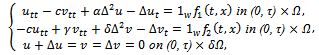 where Ω is a sufficiently regular bounded domined in
  and
and  such that
  ,ω is an open nonempty subset of Ω, 1ω denotes the characteristicfunction of the set ω and the distributed control
  . Specifically, we prove the following statement: For all
  the system is approximatelycontrollable on
  . Moreover, we exhibit a sequence of controls steering thesystem from an initial state to a
  final state in a prefixed time
 .
.
Keywords:
Interior Controllability, Timoshenko Type Equation, Strongly Continuous Semigroups
Cite this paper:
Hanzel Lárez , Hugo Leiva , Darwin Mendoza , "Interior Controllability of a Timoshenko Type Equation", International Journal of Control Science and Engineering, Vol. 1 No. 1, 2011, pp. 15-21. doi: 10.5923/j.control.20110101.03.
1. Introducción
The Timoshenko beam theory was developed by Ukrainian-born scientist Stephen Timoshenko in the beginning of the 20th century. The model takes into account shear deformation and rotational inertia effects, making it suitable for describing the behavior of short beams, sandwich composite beams or beams subject to high-frequency excitation when the wavelength approaches the thickness of the beam. The resulting equation is of 4th order, but unlike ordinary beam theory - i.e. Bernoulli-Euler theory, there is also a second order spatial derivative present. Physically, taking into account the added mechanisms of deformation effectively lowers the stiffness of the beam, while the result is a larger deflection under a static load and lower predicted eigenfrequencies for a given set of boundary conditions. The latter effect is more noticeable for higher frequencies as the wavelength becomes shorter, and thus the distance between opposing shear forces decreases. This paper has been motivated by the works in[2],[8],[9],[10],[12] and[13], where a new technique is used to prove the approximate controllability of some diffusion process.Following[2],[9] and[13], in this paper we study the interior approximate controllability of the following Timoshenko Type Equation | (1) |
Where Ω is a sufficiently regular bounded domain in  and
and  such that
  , ω is an open nonempty subset of
  , denotes the characteristic function of the set ω and the distributed control
  Specifically, we prove the following statement: For all
  the system is approximately controllable on
 Moreover, we exhibit a sequence of controls steering the system from an initial state to a final state in a prefixed time
  But, before proving this result, we study the approximate controllability of the following Timoshenkotype equation with the controls acting in the whole set Ω using some result from[8].
 | (2) |
Where .Of course, the interior approximate controllability of this equation is more interesting problem from the applications point of view since the control is acting only in a subset or part of Ω. Our technique is simple and rests on the shoulders of the following fundamental results:Theorem 1.1.[10] The eigenfunctions of -Δ withDirichlet boundary condition on
  are real analytic functions.Theorem 1.2.[1]Suppose
  is an open, nonempty and connected set, and f is areal analytic function in Ω with
  on a non-empty open subset ω of Ω. Then
  in Ω.
in Ω.
2. Abstract Formulation of the Problem
Let  and consider the linear unbounded operator
 defined by
  , where
  | (3) |
The operator A has the following very well known properties: the spectrum of A consists of only eigenvalues ,each one with multiplicity
  equal to the dimension of the corresponding eigenspace.a) There exists a complete orthonormal set
  of eigenvectors of A.b) For all
  we have
 | (4) |
Where is the inner product in X and
 | (5) |
So,  is a family of complete orthogonal projections in z and
 | (6) |
c)  generates an analytic semigroup
 given by
 | (7) |
d) The fractional powered spaces  are given by:
 ,with the norm
 ,And
,And | (8) |
Also, for  we define
 , which is a Hilbert Space with norm givenby
 Hence, the equations (1) and (2) can be written as abstract systems of ordinary differential equations in the Hilbert space
 | (9) |
 | (10) |
where | (11) |
and | (12) |
is a linear unbounded operator with domain  and
and Now, using the following Lemma from[11] we can prove that the linear unbounded operator
  given by the linear equation (9) generates a strongly continuous semigroup which decays exponentially to zero.Lemma2.1.Let Z be a separable Hilbert space and
  two families of bounded linear operators in Z with
  being a complete family of orthogonal projections such that
 | (13) |
Define the following family of linear operators | (14) |
Thena) T(t) is a linear bounded operator if | (15) |
for some continuous real-valued function g(t).b) Under the condition (15)  is a C0 -semigroup in the Hilbert space Z whose infinitesimal generator
  is given by
 | (16) |
With | (17) |
c) The spectrum  of
of  is given by
 | (18) |
Theorem 2.2.The operator  given by (12) is the infinitesimal generator of a strongly continuo semigroup
 represented by
 | (19) |
Where is a complete family orthogonal projections in the Hilbert space
  given by
 | (20) |
and | (21) |
Where  Therefore,
  , the ingenvalues
 are simple and
 Where
Where are the roots of the characteristic equation
 and this semigroup decays exponentially to zero; that is to say,
 where
where and
and The following gap condition plays an important role in this paper
 | (22) |
3. Controllability of the System (10)
In this section we shall prove the approximate controllability of the system (10). But, before we shall give the definition of approximate controllability for this system. To this end, for all  and
and  the initial value problem
 | (23) |
were  , admits only one mild solution given by
  | (24) |
Definition 3.1.(Approximate Controllability) The system (10) is said to be approximately controllable on  if for every
  there exists
  such that the solution
  of (23) corresponding to
  verifies:Definition 3.2. For the system (10) we define the following concepts:a) The controllability mapping
  is defined by
  | (25) |
b) The grammian mapping  is given bythat is to say
 Theorem 3.3.The system (10) is approximately controllable on
  if, and only if, one of the following statements holds:
 Proposition 3.4.The following equality holds:
 | (26) |
Prof.From (11) we know that  Then,
Then,  And
And  Since
Since  we get that
 On the other hand,
 Therefore,
 REMARK 3.1.If ω is a nonempty open sub set of Ω such that
  , then
 Now, we shall use the equality (26) in order to characterize the approximate control ability of the system (10) in terms of the following family of finite dimensional control problems,
 | (27) |
where Proposition 3.5. The operator
 can be written as follows
 where,
 Proof. From condition (26) and the representation (19) of T(t) we obtain
 where,
 Theorem 3.6.a) The system (10) is approximately controllable on
  if, and only if, each of the following system
 | (28) |
is approximately controllable.b)The system (10) is approximately controllable on  if, and only if
 Proof.a) For the purpose of contradiction, let us assume that system (10) is approximately controllable on
  and there exists j such that the system
 is not approximately controllable on
 . Then, there exists
  such that:
 | (29) |
On the other hand, from part (iii) of Theorem 3.3 we have that: Now, letting
  , we obtain:
 This implies that
 , which contradicts the assumption. Therefore, (28) is approximately controllable for all j.If for all j system (28) is approximately controllable, then by Theorem 3.3 part (ii),
 Clearly that, for all
  , there exists
  such that
 . Then, using Proposition 3.5, we get for all z in Z that
 Hence, (10) is approximately controllable and (a) is proved.b) follows immediately from (a) and Theorem 3.3.Next, we shall use the following result: Consider the following finite dimensional controlsystem
 | (30) |
Where A and B are matrixes of dimensions  and
and  respectively.Theorem 3.7. (see[Lee and Marcus(1967)]). (Kalman) The system (30) is controllably on
  if, and only if,
 That is to say,
 where
where  is the vector space generated by
  .Theorem 3.8. The system (10) is approximatelycontroll-able on
 .Proof. It is enough to prove the controllability of the finite dimensional system (28) with
 and
and So,
So, where
where Therefore, the controllability of the system (28) is equivalent to the controllability of each finite dimensional systems,
 | (31) |
where, and the system (31) is controllable if, and only if,
 which can be verified trivially. Therefore, system (31) is controllable, and consequently, system (10) is also approximately controllable applying Theorem 3.6.
4. Proof of the Main Theorem
In this section we shall prove the main result of this paper on the approximate controllability of the linear system (9). To this end, we observe that the definition of controllability for system (9) is similar to the one given to system (10). And, for all  and
and  the initial value problem
 | (32) |
admits only one mild solution given by | (33) |
Consider the following bounded linear operator: | (34) |
Whose adjoint operator  is given by
 | (35) |
The following lemma is trivial:Lemma 4.1.The equation (9) is approximately controllable on  if, and only if,
 .The following result is well known from linear operator theory:Lemma 4.2.Let W and Z be Hilbert spaces and
  the adjoint operator of the linear operator
  . Then,
 As a consequence of the foregoing Lemma one can prove the following result:Lemma 4.3.Let W and Z be Hilbert spaces and
  the adjoint operator of the linear operator
 Then
Then  if, and only if, one of the following statements holds:
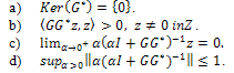 The following theorem follows directly from (35), lemma 4.1 and lemma 4.3.Theorem 4.4.(9) is approximately controllable on
  if, and only if,
 | (36) |
For the proof of the main theorem of this paper we shall use the following version ofLemma 3.14 from [3] and Lemma 4.4 from [2].Lemma 4.5.Let be sequences of real numbers such that
 | (37) |
Then, for any  we have that
 | (38) |
if, and only if, | (39) |
Proof. (Lemma 4.5) By analytic extension we obtain | (40) |
Now, dividing this expression by we get
 From (37) we have that
  and
and  for
for  and
and , for
, for , then passing to the limit when
  we obtain that
 .Then, we have that
 Now, dividing this expression by
  we get
 From (37) we have that
  and
and  for
for  and
and , for
, for  , then passing to the limit when
  we obtain that
 .Then, we have that
 In general, if we continue with this process and divide this expression by
 , we get that
 From (37) we have that
 Then, passing to the limit when
  we obtain that
  So, continuing with this procedure we get that
 and
and Repeating this procedure from here, we would obtain that
 ,and continuing this way we get
  Now, we are ready to formulate and prove the main theorem of this work.Theorem 4.6.(Main Result) For all nonempty open subset ωof Ω and
  the system(9) is approximately controllable on
 . Moreover, a sequence of controls steering thesystem (9) from initial state
  to an
to an  neighborhood of the final state
  at time
  is given by
 and the error of this approximation
  is given by
 Proof. We shall apply Theorem 4.4 to prove the controllability of system (9). To this end, we observe that
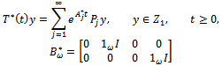 and, since the eigenvalues of the matrix
  are simple, there exists a family of complete complementary projections
  such that
 Therefore,
 where
where  Now, suppose that
  . Then,
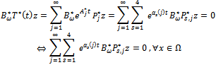 The assumption (22) implies that the sequence
 satisfies the conditions on Lemma 4.5. In fact, we have trivially that
  for
for  and from (22) we obtain:
 Therefore,
 Then, from Lemma 4.5 we obtain for all
  that
that Since
Since we obtain that,
 Then,
Then, On the other hand, from Theorem 1.1 we know that
  are analytic functions, which implies the analyticity of
 . Then, from Theorem 1.2 we get for
  that
that From Theorem 3.8, the system (10) is approximately controllable. So, from part iii) of Theorem 3.3 we conclude that
  .Therefore,
 Then, from Theorem 4.4 we obtain that system (9) is approximately controllable.Now, given the initial and the final states
  and
and , we consider the sequence of controls
 Then,
Then, From part c) of Lemma 4.3 we know that
 Therefore,
 This completes the proof of the Theorem.Corollary 4.7.The approximate controllability of the system (9) is equivalent to the approximate controllability of the system (10).
5. Final Remark
The result presented in this paper can be formulated in a more general setting. Indeed, we can consider the following Timoshenko Type Equation in a general Hilbert space Z and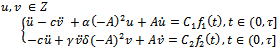 | (41) |
where,  is an unbounded linear operator in Z with the spectral decomposition given by
 with eigenvalues
 each one with multiplicity
  equal to the dimension of the corresponding eigenspace.a) There exists a complete orthonormal set
  of eigenvectors of A.b) For all
  we havec)
  | (42) |
The controls  and
and  are linear and bounded.When
  , the operators
  and
and  are particular cases of
  and
and .
.
References
| [1] | S. Axler, P. Bourdon and W. Ramey, Harmonic Fucntion Theory. Graduate Texts in Math., 137. Springer Verlag, New York (1992). |
| [2] | Salah Badraoui, Approximate Controllability of a Reaction-Diffusion System with a Cross Diffusion Matrix and Fractional Derivatives on Bounded Domains, Journal of Boundary Value Problems, Vol. 2010, Art.ID 281238, 14pgs.(2010). |
| [3] | R.F. Curtain, A.J. Pritchard, Infinite Dimensional Linear Systems. Lecture Notes in Control and Information Sciences, 8. Springer Verlag, Berlin (1978). |
| [4] | R.F. Curtain, H.J. Zwart, An Introduction to Infinite Dimensional Linear Systems Theory. Text in Applied Mathematics, 21. Springer Verlag, New York (1995). |
| [5] | Luiz A. F. de Oliveira, On Reaction-Diffusion Systems” E. Journal of Differential Equations, Vol. 1998(1998), N0. 24, pp. 1-10. |
| [6] | Jong Uhn Kim, On the Energy Decay of a Linear Thermoelastic Bar and Plate. SIAM J. Math Anal.Vol.23, No. 4, pp 889, (1992). |
| [7] | J. Lagnese, Boundary Stabilization of Thin Plate. SIAM Studies in Appl. Math.10, Philadelphia. Controllability of Timoshenko Type Equation. 17,(1989). |
| [8] | H. Lárez, H. Leiva and J. Uzcátegui, Controllability of Block Diagonal Systems and Applications, Int. J. Systems, Control and Communications, Vol. 3, No. 1, (2011). |
| [9] | H. Lárez and H. Leiva, Interior controllability of a 2£2 reaction-diffusion system with cross-diffusion matrix, Boundary Value Problems, Vol. 2009, Article ID560407, 9 pages, doi:10.1155/2009/560407. |
| [10] | H. Leivaand Y. Quintana, Interior controllability of a broad class of reaction diffusion equation, Mathematical Problems in Engineering, Vol. 2009, Article ID708516, 8 pages, doi:10.1155/2009/708516. |
| [11] | H. Leiva, A Lemma on C0-Semigroups and Applications PDEs Systems Quaestions Mathematicae, Vol. 26, pp. 247-265 (2003). |
| [12] | H. Leiva, A necessary and sufficient algebraic condition for the controllability of thermoelastic plate equation, IMA Journal of Control and Information, pp.1-18, (2003). |
| [13] | H. Leivaand N. Merentes, Interior controllability of the thermoelastic plate equation, African Diaspora Journal of Mathematics, Vol. 12, N. 1, pp. 1-14 (2011). |
| [14] | Y. Shibata, On the Exponential Decay of the Energy of a Linear Thermoelastic Plate. Comp. Appl. Math. Vol. 13, No. 2, pp. 81-102,(1994). |
 Abstract
 Reference
 Full-Text PDF
 Full-Text HTML