Tarini Mishra
Northwest Missouri State University, Maryville MO, USA
Correspondence to: Tarini Mishra, Northwest Missouri State University, Maryville MO, USA.
| Email: |  |
Copyright © 2024 The Author(s). Published by Scientific & Academic Publishing.
This work is licensed under the Creative Commons Attribution International License (CC BY).
http://creativecommons.org/licenses/by/4.0/

Abstract
In today’s highly selective marketing world, analysing customer behaviour and preferences is one of the key attributes in defining successful marketing and advertising campaigns. Deriving relevant insights from marketing data which is collected across multiple touch points will enable marketers to create relevant advertising and marketing campaigns across relevant channels maximising their return on investment. Additionally, AI/ML tools which can be deployed on these data will make marketers smarter by enabling them to predict customer behaviour and designing campaigns accordingly. We have analyzed few ML methodologies in this report and have derived an equation of linear regression for marketers to predict customer purchases based on their income. We have also analyzed statistical data to compare performances of campaigns and channels. Our analysis shows how campaigns have matured over time and how store purchases lead over other channels to keep brick and motor stores relevant over web transactions. These findings will help marketers design their campaigns so that they can target their customers at the right channel, at the right time with the right content.
Keywords:
Marketing Analytics [1], Data Analytics, Machine Learning, Data Cleansing, Marketing Campaigns, Marketing Channels, Predictive Analytics, Linear Regression, Neural Networks, Random Forest
Cite this paper: Tarini Mishra, Marketing Analytics - Campaigns Influence on Consumer Preferences Across Channels, Computer Science and Engineering, Vol. 14 No. 5, 2024, pp. 98-107. doi: 10.5923/j.computer.20241405.02.
1. Introduction
I have choosing Marketing domain as it is inline to my profession. I have choosen my datset from Kaggle website. The link to the data source is https://www.kaggle.com/datasets/jackdaoud/marketing-data. This data source has de- tails about customer profiles and their product preferences which can be analyzed on the attributes like campaign performance across channels.The problem I am trying to analyze is to figure out how campaign performance across channels impact product preferences for different customer profiles. This is important in real world as it will analyze the impact of campaigns and channels on customer preferences for different products and how it can impact transformation in consumer behaviour. [1]Below are the steps or phases of your project implementation:1. Finalizing Dataset and preparing Github Repo2. Identifying the key parameters for analysis3. Data preparation and cleansing4. Planning and building the model5. Operationalizing the model and capturing the resulting analytics6. Submitting finalized latex and pdf report using OverleafKey components of my approach are Data cleansing and Machine Learning model which will lead me to my analysis.
1.1. Sections of This Project
- Data Collection- Data Cleansing- Exploratory Data Analysis- Predictive Analytics- Models Evaluation Results- Conclusion
2. Data Collection
2.1. Data Source
My Data source is https://www.kaggle.com/datasets/jackdaoud/marketing-data.
2.2. Data Format
The format of the data source is CSV and I imported the data source as it is, in CSV format.
2.3. Data Scraping
The data was available in a structured manner and I did not have to use any Data scraping technique to extract information. I imported the CSV in python code and use panda library to read the attribute values.
2.4. Data Attributes to be Used for Analysis
Few of the important attributes which I used as a part of this analysis is Income, NumStorePurchases, NumCatalogPurchases, NumWebPurchases, NumWebVis- itsMonth, NumDealsPurchases, AcceptedCmp5, AcceptedCmp4, AcceptedCmp3, AcceptedCmp2, AcceptedCmp1, AcceptedCmpOverall, Age, educationbasic, educationGraduation, educationMaster, educationPhD to list a few.
2.5. Data Extraction
We did a one time import of the full data set using Panda libraries directly from the source - Kaggle site. As the data is already structured and transformed to a huge extent, we used the data as it is for our analysis.
3. Data Cleaning
3.1. Data Cleaning Process
Although I have chosen a structured data set but I have to undergo the process of Data Cleaning and Transformation.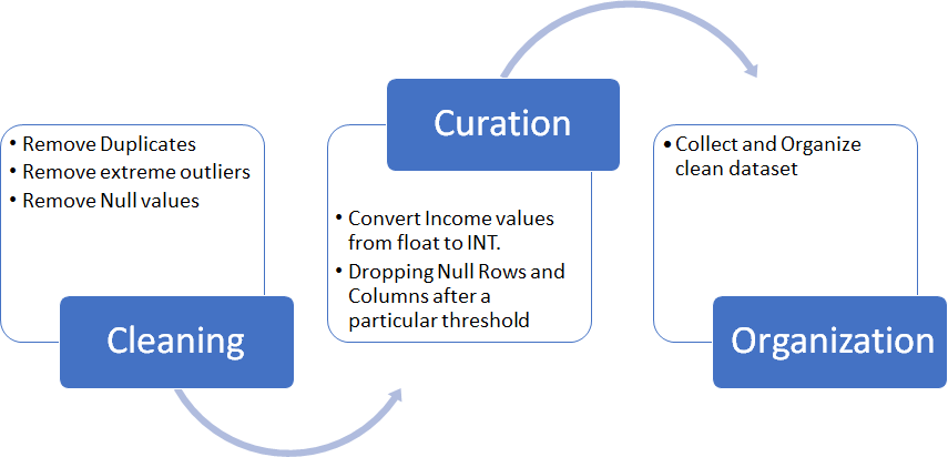 | Figure 1. Data Cleaning Process [4] |
3.2. Tools and Techniques to be Used for Data Cleaning
- For removing duplicates we used drop duplicate()- For checking Null values we used isnull.any() functioning for dropping null rows we will be using dropna(thresh=thresh, axis = 1).shape- For removing extreme outliers we used Quantile function with operator- We used INT() function to convert Income values from float to INT
3.3. Missing Value Strategy
Isnull.any() will check for missing values and dropna() will remove the row with the null value.
3.4. Data Attributes and Record Count after Cleaning Process
My data data attributes remain the same I.e 2206 Rows and 39 columns as I choose a structured set and none of my attribute had missing values.
3.5. Definitions of Important Data Attributes
We will be using selected attributes from our dataset in our analysis to derive findings. Below are the list of attributes which will be important for our EDA and our results:- Income: This is one of the most important attribute which we used for our analysis in consumer behavior.- Age: Age is used to determine the category of products consumed by different age groups.- NumOfWebVisitispermonth: This attribute helps us analyze if the website influenced any purchase behavior.- MntTotal: This is the total products consumed and this attribute will be used as a denominator for other products.- AcceptedCmpOverall: Total number of campaign accepted by the consumer which might influence purchase behavior.- MnRegularProducts: This is the total number of regular products consumed.- Education basic: This identifies if a consumer has basic level education which might influence purchase behavior.- Education Master: This identifies if a consumer has master level education which might influence purchase behavior.- Education Graduation: This identifies if a consumer has Graduation level education which might influence purchase behavior.- Education Phd: This identifies if a consumer has PHD level education which might influence purchase behavior.- Marital Single: This identifies if a consumer’s marital status is single which might influence purchase behavior.- Marital Divorced: This identifies if a consumer’s marital status is divorced which might influence purchase behavior.- Customer Days: This attribute defines if loyalty of consumer impacts purchase behavior.
3.6. Dependent and Independent Variables for the Analysis
MntTotal is a dependent variables related to consumer behavior analysis. Income, AcceptedCmpOverall, Education and Marital status are independent variables for our analysis.
4. Exploratory Data Analysis
Exploratory Data Analysis (EDA) is a methodology which helps identify the understand the data model and identify co-relations and pattern between the data attributes. It is very essential in a data science or data analytics project as it reveals essential characteristics of the dataset which eventually helps in holistic data insights.
4.1. Exploratory Data Analysis Technique
Below are primary types of EDA techniques:- Univariate nongraphical - Multivariate nongraphical - Univariate graphical- Multivariate graphicalHistograms and Box plots are going to help comprehend the relationships and identify outliers. So Univariate graphical technique will work for my project. I will also leverage Multivariate graphical technique when and where required.
4.2. Preliminary Results of Exploratory Analysis
This technique helped me identify the characteristics of these important data attributes. For ex:- The Average age range doing the transactions- Average customer days- Income range of the surveyed customer- Graduated vs basic profiles- Marital statusExploratory Data Analysis phase helps understand the various data attributes and what kind of relationship I can generate between Customer Profile, Education and Marital Status. It also helps identify the campaign acceptance based on profiles which is key to this analysis. This phase gave me an idea about the ideal range of values for each profile attribute. I will continue with my analysis for deeper insights on purchase behavior and link them to the profile attribute.
4.3. Specifics of Processing
Below are the sequence of activities which we performed as a part of EDA:- Converted Income column from Float to Int to deal with whole numbers- Removed the Outliers for teh accuracy of the analysis- Identified customer profile data attributes and created histogram for each attribute - Income, Age, Dt Customer, Recency, Kidhome, Teenhome- Identified Education related and created histogram for each attribute - education Basic, education Graduation, education Master, education PhD- Identified Marital status attributes and created histogram for each attribute - marital Divorced, marital Married, marital Single, marital Together, marital Widow
4.4. Code Snapshot
Removing Null values:thresh = len(data _frame)*0.6 data _frame.dropna(thresh=thresh, axis = 0).shape(Converting Income from Float to Int:data _frame.Income.value _counts() data frame[’Income’] = data _frame[’Income’].apply(int) data _frame.Income.value _counts()Removing Extreme Outliers:data _frame _outliers = data _frame[(data _frame.Income ¡ data _frame.Income.quantile(0.995)) (data _frame.Income ¿ data _frame.Income.quantile(0.005))] data _frame _outliers.hist(’Income’)Sum of food purchased:data _frame[’MntTotal’] = data _frame.loc[:,[’MntWines’, ’MntFruits’, ’MntMeat-Products’, ’MntFishProducts’, ’MntSweetProducts’]].sum(axis=1) data _frame.MntTotal.head()Histograms:data _frame.hist(column = [’Age’, ’Customer Days’, ’Income’, ’Kidhome’, ’Teen- home’], figsize=(45,25))Histograms showcase the mean values for each attribute of the customer profile - Age, Customer Days, Income, Kidshome and Teenhome. We will have boxplots for these customer profiles in Section 6 of the report, where we will explain our analysis. For detailed code, please visit my My Github Repo.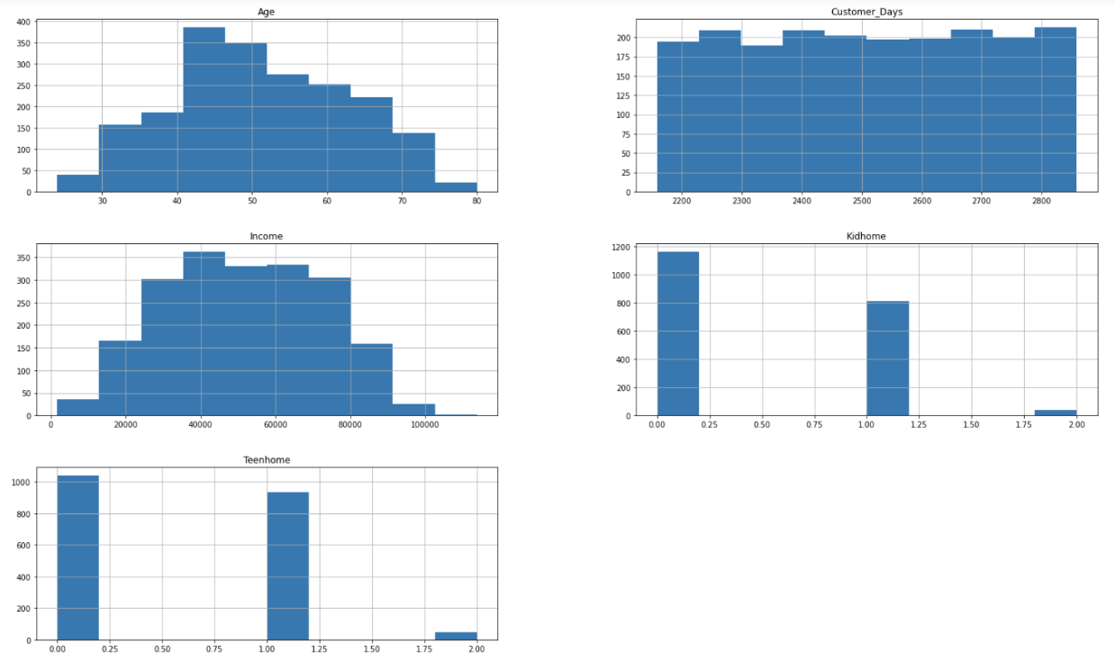 | Figure 2. Histograms |
4.5. Exploratory Data Analysis Findings
Exploratory Data Analysis phase helps us understand the various data attributes and what kind of relationship I can generate between Customer Profile, Education and Marital Status. It also helps me identify the campaign acceptance based on profiles which will be the key to this analysis. This phase gave me an idea about the ideal range of values for each profile attribute. We continue with our analysis for deeper insights on purchase behavior in the following sections and link them to the profile attribute.
5. Predictive Analytics
5.1. Analysis Technique
Creating a pipeline for predictive application [5] is all about automating the data ingestion and processing the data models for desired outcome. This helps in maintenance of the overall system with reduced effort. The model I am trying to follow can be depicted with the below diagram: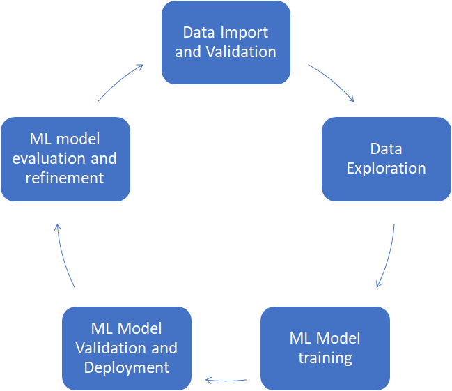 | Figure 3. ML Automation process [4] |
1. Data Import and Validation - We are not continuously streaming data so we will do a one time import of the data which will be validated before processing.2. Data Exploration: Essential information was extracted from the ingested data which will help us understand and predict the data.3. ML Model Training: A model is selected and data is transformed into test and train data sets.4. ML Model Validation and Deployment: After the predictions are verified for the targeted values the Model is deployed.5. ML model evaluation and refinement: Predictions are constantly monitored to improve the ML Model.
5.2. Machine Learning Algorithms
We are using multiple ML algorithms to analyze the data and eventually select the best performing one to make predictions:1. Linear Regression2. Random Forest3. Neural Network
5.3. Training and Testing Process
For training and testing phase of the data, We had to split the data 80-20 using train test split library. As it is a one time imported data, we will do this partition once. Training set will be used for building the predictive model and testing set will be used for actual predictions. We will be applying multiple ML algorithms to choose the best model amongst all of them. | Figure 4. 80-20 train-test split of dataset |
5.4. ML Algorithms Implementation
We have identified 3 different ML algorithms for building my model on the training set.Linear Regression: We will evaluate this supervise learning method to determine any linear relationships between Income and Purchase considering Campaign acceptance.Random Forest: This algorithm is a type of ensemble learning which generally has less bias and variance as it is an extension of classification and regression decision and combines multiple decision trees.Neural Network: This deep learning technique will give us result like hu- man brain processing which will be different than other ML learning models.Once we have defined the models, we are going to evaluate the accuracy of these 3 models by comparing the Bias and Variance for Linear Regression. For Neural Network and Random Forest we will be comparing Accuracy and Precision to determine the preferred model.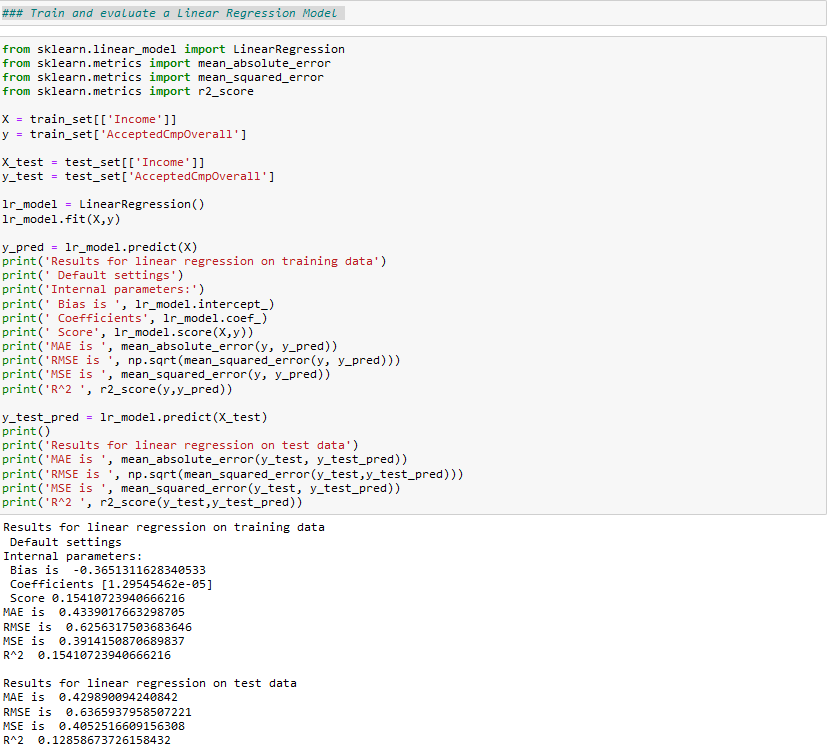 | Figure 5. Linear Regression Test and Train model with resulting Bias, Coefficients, Score, Mean Absolute Error and Mean Squared Error |
6. Models Evaluation Results
Basic results for our classification model to predict Campaign Acceptance based on Income and Total PurchaseModel— Training Features— Acc Train— F1 Train— Acc Test— F1 Test Neural Network— ’Income’, ’MntTotal’ — 78—69—80.74—72.13Random Forest— ’Income’, ’MntTotal’ —100—100—77.28—74.72Random Forest looks to be overfitting with the Training statistics as com- pared to the Neural Network model.Results on Linear Regression:Bias is -0.3651311628340533Coefficients [1.29545462e-05] Score 0.15410723940666216Data type — MAE — RMSE — MSE — R2 Train data — 0.43 — 0.62 — 0.39 — 0.15Test data — 0.42 — 0.63 — 0.40 — 0.12We prefer Linear regression over classification models as the error rate is minimal. This Linear regression model shows the Campaign acceptance percent- age based on Income variable. Below screenshot shows the linear slope of the equation.The linear regression prediction model is y = Coefficient (X) + Bias (C). So our model will have a prediction equation y = [1.29545462e-05]X + [-0.365], where Y is the total amount of purchase and X is the Income value. Based on this equation, household purchase predictions can be made for other customers using their income.For detailed code, please visit my My Github Repo.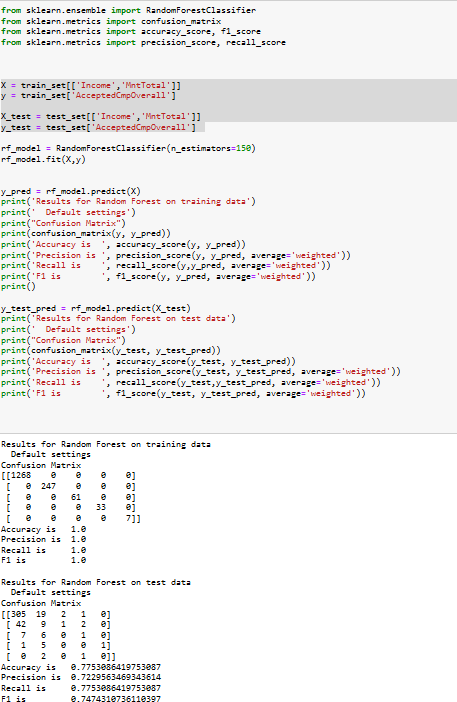 | Figure 6. Random Forest Test and Train model with resulting scores of Accuracy, Preci- sion, Recall and F1 |
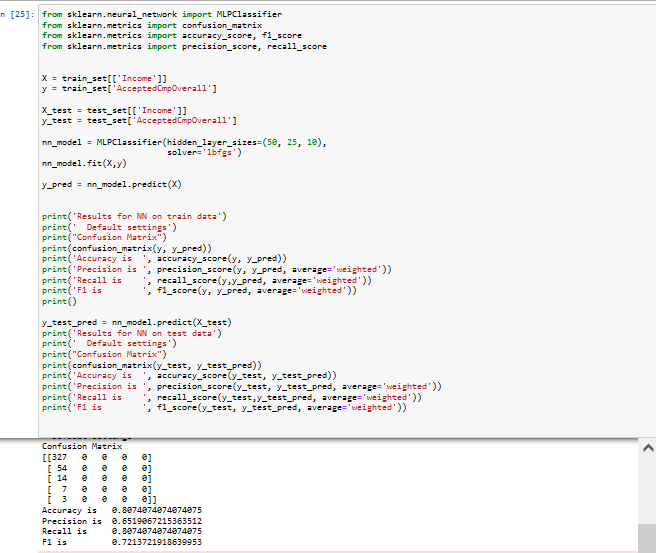 | Figure 7. Neural Network Test and Train model with resulting scores for Accuracy, Pre- cision, Recall and F1 |
7. Conclusions
The problem we are trying to analyze is to figure out how campaign performance across channels impact product preferences for different customer profiles. This is important in real world as it will analyze the acceptance of campaigns impacts customer preferences for different products with their income. Our data source has details about customer profiles and their product preferences which can be analyzed on the attributes like campaign performance across channels. Our Linear Regression slope shows a direct correlation between Income and Number of Accepted campaigns. Surveyed people with higher income tend to accept more campaigns resulting in higher purchase.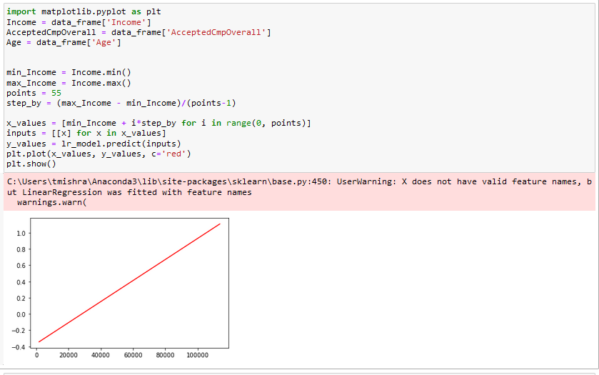 | Figure 8. Slope resulting from the equation of the linear regression model |
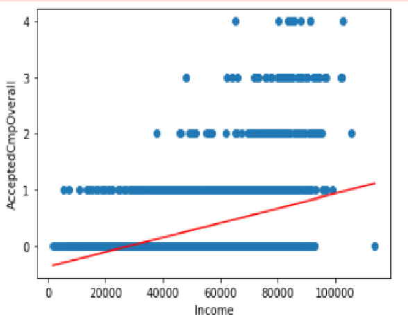 | Figure 9. Linear Slope |
Figure 10 bar graph shows the relationship of the number of Web Visits to the number of deals purchased. It cannot be concluded that high number of web visits is resulting in higher number of deals purchased.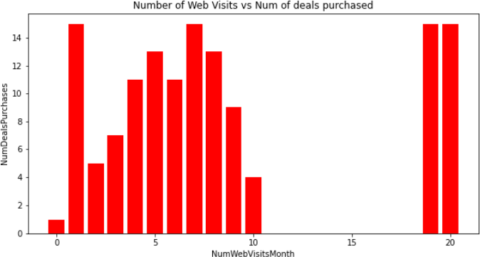 | Figure 10. Web visits vs deals purchased |
Figure 11 Bar graph shows the relationship between number of dependents (Kids and Teens) in an household with the number of stores purchased. House- holds with Teens and Kids do tend to make frequent store purchases.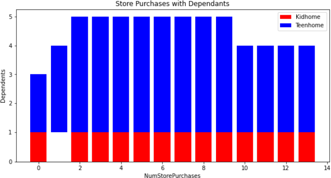 | Figure 11. Households with Kids and Teens |
For detailed code, please visit my My Github Repo.
7.1. Conclusions Based on Statistical Evidence
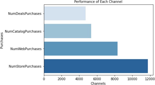
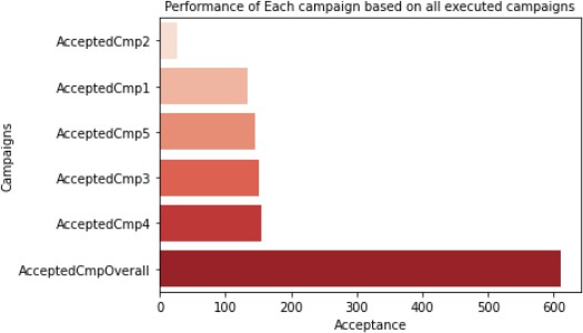
Based on the statistical evidence across all channels [2], Store Purchases outper- form all other channels of purchase. Below seaborn plot in figure 13 compares the Store purchases with the Web Purchases, Catalog Purchases and Deals Purchases. Store Purchases is a clear winner followed by Webpurchases. Please see the code snippet used to create the Horizon Bar plots.Based on the statistical evidence For campaigns, newer campaigns have higher acceptance as compared to the older campaigns executed previously. Below seaborn plot compares all the campaigns vis a vis total number of accepted campaigns. Barplot on figure 15 clearly shows that Campaign no. 4 has highest acceptance and campaign no. 2 has the least acceptance. Please see the code snippet used to create the Horizon Bar plots. | Figure 12. Channel Performance Comparison plotting |
 | Figure 13. Channels Performance |
 | Figure 14. Campaign Performance comparison plotting |
 | Figure 15. Campaign Performance |
For detailed code, please visit my My Github Repo.
7.2. Limitations
Limitations of this project:- Data collected is only for Food items- Data has only 2206 observations
7.3. Future Work Recommendations
“As customers go through a series of touch points across media, channels and devices on their paths to purchase understanding the effectiveness of each touch point and their complementary roles in leading to overall conversions is becoming very important” [3]. As future work I recommend to analyze how each of the campaign is impacting the purchase decisions or campaign acceptance, which will be a deeper analysis for combination of the below graphs: | Figure 16. Channels and Campaigns |
Ethical Declaration
Not applicable.
References
| [1] | Bakopoulos, V., Stuart, G., Briggs, R.: Measuring the value of mobile advertising in driving business outcomes: Empirical data from coca-cola, at&t, mastercard and walmart. Applied Marketing Analytics 2(2), 169–179 (2016). |
| [2] | Furey, T., Friedman, L.: The channel advantage. Routledge (2012). |
| [3] | Kannan, P., Reinartz, W., Verhoef, P.C.: The path to purchase and attribution modeling: Introduction to special section (2016). |
| [4] | Mishra, T.: Campaigns influence on consumer preferences across channels (2023). |
| [5] | Murgai, A.: Transforming digital marketing with artificial intelligence. International Journal of Latest Technology in Engineering, Management & Applied Science 7(4), 259–262 (2018). |


 Abstract
 Reference
 Full-Text PDF
 Full-text HTML