Jay P. Narain
Retired, Worked at Lockheed Martin Corporation, Sunnyvale, CA, USA
Correspondence to: Jay P. Narain, Retired, Worked at Lockheed Martin Corporation, Sunnyvale, CA, USA.
| Email: | 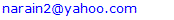 |
Copyright © 2021 The Author(s). Published by Scientific & Academic Publishing.
This work is licensed under the Creative Commons Attribution International License (CC BY).
http://creativecommons.org/licenses/by/4.0/

Abstract
The solution of Partial differential equations has been of considerable interest lately because of interest in Machine Learning methods [1,2,3]. The use of artificial neural network to solve ordinary and elliptic partial differential equations has been elaborately described in these papers. Presently some of the salient features of a new simpler artificial neural network has been investigated. While in this neural network one can introduce random grid points and modelling errors, the solutions presented in the paper show that the new ANN scheme is both able to minimize the modelling errors and increase solution efficiency of elliptic partial differential second order equations.
Keywords:
Differential equations: Elliptical partial, Neural netwok, Network differentiation, Machine learning methods
Cite this paper: Jay P. Narain, Efficiently Solving Poisson’s Equation Using Simple Artificial Neural Networks, Computer Science and Engineering, Vol. 11 No. 2, 2021, pp. 23-27. doi: 10.5923/j.computer.20211102.01.
1. Introduction
The neural network schemes require derivative of neural network. The autograd library [4] provides excellent automatic differentiation scheme. Angel [5] has developed a nice scheme for multi -dimensional neural network and their derivatives. With this scheme, any first and second order partial differential equation can be solved with ease. In the present analysis, we will investigate the effect of modelling error on the final outcome. Next, we will examine effect of random point distribution on the numerical solution. Lastly, we will solve the equation in irregular domain.
2. Discussions
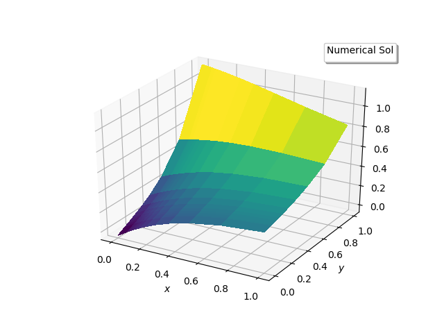
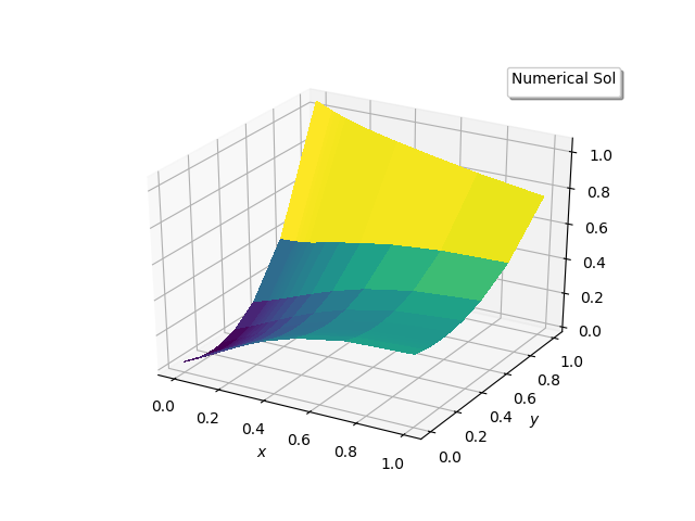
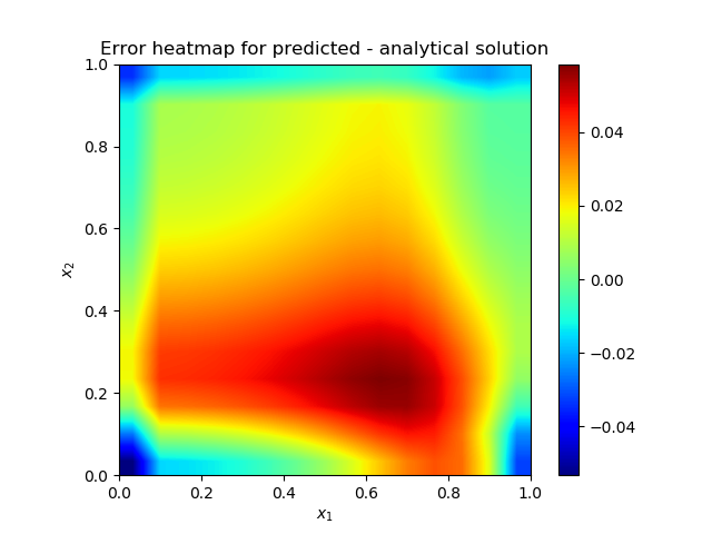
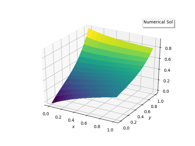
(A) The solution of partial differential equations by Artificial Neural Network (ANN) has become very routine. They are many outstanding works in this field using various concepts [1,2,3]. We will be following boundary condition-based solution of Poisson’s equation method [3]. The automatic differentiation scheme of neural network will be used, [5] The basic model of the study for reference is as follows:Exact Contrived solution: 𝛟 = exp(-x)*(x+y3)Source term(right hand side of Poisson’s eq.): f = exp(-x)*(x-2+y3+6*y)Laplace operator (left hand side eq.): d2 𝛟(x,y)/dx2 + d2 𝛟(x,y)/dy2 Boundary conditions: Dirichlet or Neumann. Used Dirichlet boundary conditions for (1,1) square domain are:bc(at y =0) = exp(-x)*xbc(at y =1) = exp(-x)*(x+1.) bc(at x=0) = y3bc(at x=1) = (1.+y3)* exp(-1.) The basic solution converges reasonably fast. The Adam [8] optimization using error loss reduction, gives a 99% converged solution in 500 iterations. Further iterations, improve the heatmap of the difference in the exact and numerical solution. About 600 secs are required for 1000 iterations on a 15x15 regularly spaced grid. The choice of hyper parameter learning rate was found critical for good prediction. Although higher values, like 0.3 show faster initial convergence but with little skewed final solution, the recommended 0.05 learning rate does the best prediction. 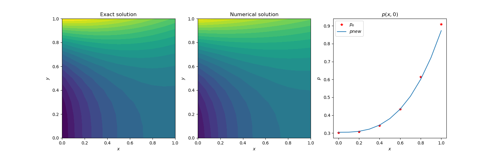 | Figure 1(a). Contour plots of exact and numerical solutions |
 | Figure 1(b). Numerical Solution |
 | Figure 1(c). Heatmap of the solution error |
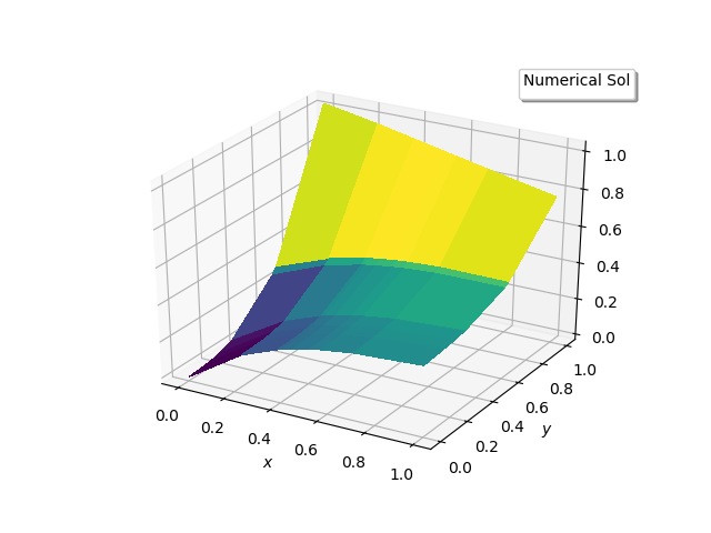
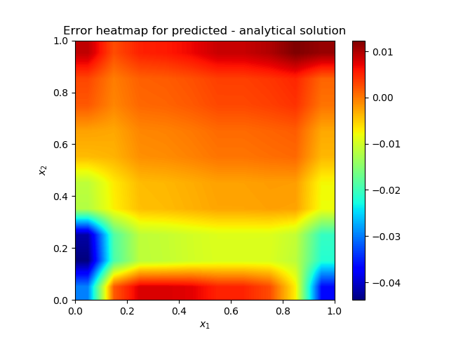
(B) The neural network works with randomly selected weights and biases for a particular problem. This method does not require any mathematical derivations, like finite difference [6], to solve the problem. The most important components are the source term and the boundary conditions. Even if the Laplace operator is set to null or calculated as null by inappropriate network differencing schemes, the optimizer converges in 500 iterations with reasonable accuracy. This is a surprising observation and should not be a common solution procedure. We tried a geometric progression 15x15 grid for this case. The following figures substantiate the observation by comparing results with the basic scheme. 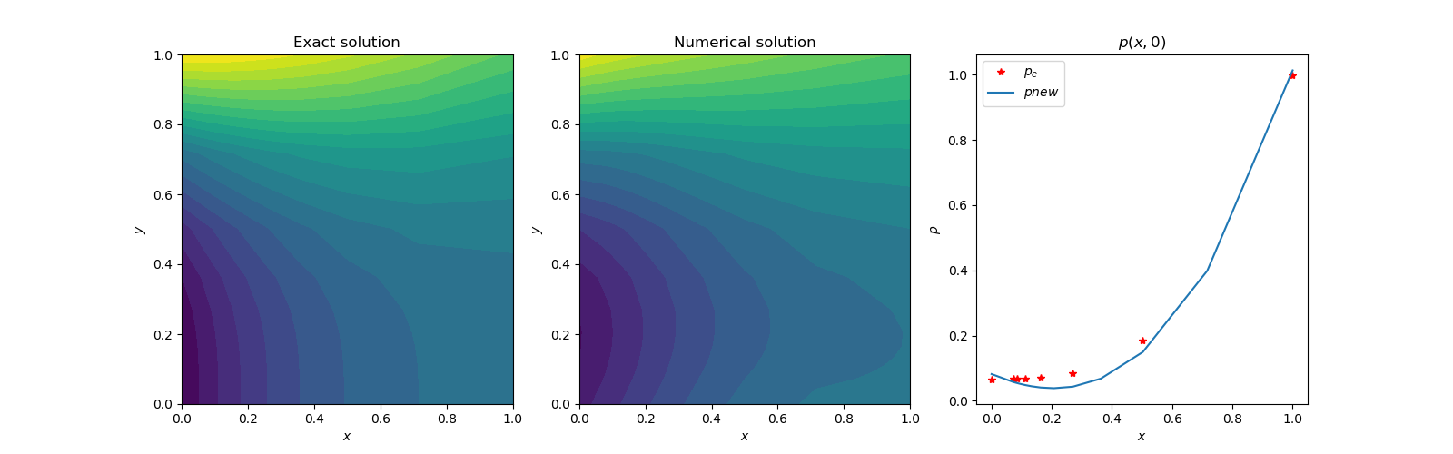 | Figure 2(a). Contour plots of exact and numerical solutions. |
 | Figure 2(b). Numerical solution |
 | Figure 2(c). Heatmap of the solution error |
(C) Since randomness is the basic part of neural network model, the random use of points in the solution domain will be a good idea. This random point distribution will avoid intricate grid generation schemes in the solution of future fluid dynamics equations. The present model problem will be solved with randomly distributed points in the domain [7]. The Laplace operator will be included in the analysis. Only the uniformly distributed random scheme will be considered. The Gaussian random distribution did not work. After the solution procedure completes, the random points have to be sorted to have customary view. The solution was carried out on 10x10 random uniform grid for 2000 iterations. The solution shows excellent results.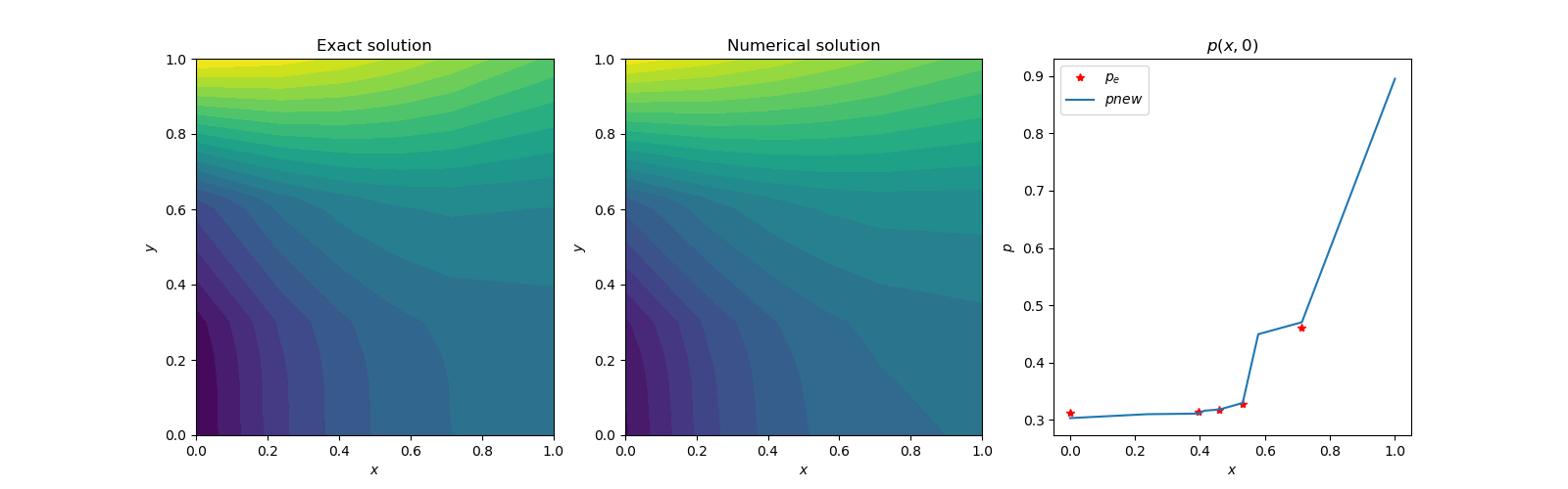 | Figure 3(a). Contour plots of exact and numerical solutions |
 | Figure 3(b). Numerical solution |
 | Figure 3(c). Heatmap of the solution error |
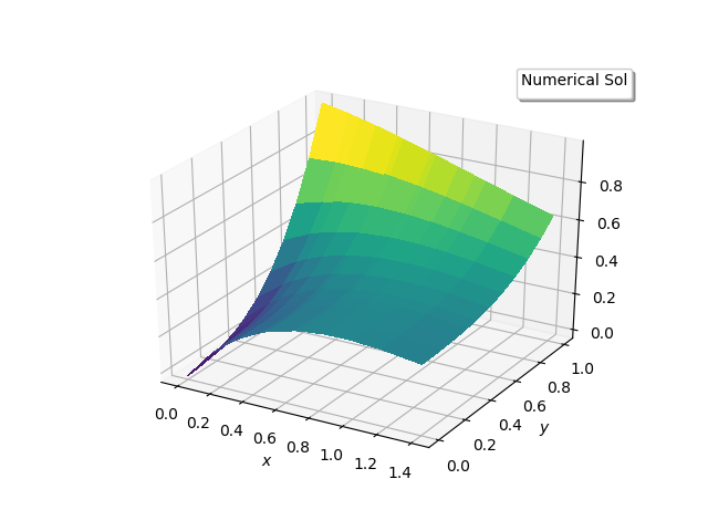
(D) Now we will consider an irregular domain. Lu Lu [2] has shown excellent result for such domain with deep learning solution method. The domain shown in Figure (4) has two partitioned domains, left as area A, right as area B. The boundary conditions are applied at all boundaries except at the interface shown in blue. This is a communication boundary condition where the values from one domain is used as the boundary condition of another domain. In fact, the left domain has (1,1) rectangular range, and the right smaller section has (.4, .4) range. The interface, shown in blue, is located at x=1.0.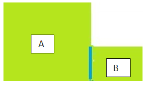 | Figure 4. L-shaped domain |
Each domain has its own neural network. Only the boundary value interchange at the interface updates their solution properly. The optimization is carried out as two simultaneous equations. Even though no specific boundary condition is applied at the interface, the exchange of field values at the interface is sufficient for the solution process to converge. Following figures show the solutions.Line plot in Figure 4(d) may look off by a big amount, but the relative error is very small as evidenced by Figure 4(f) heatmap.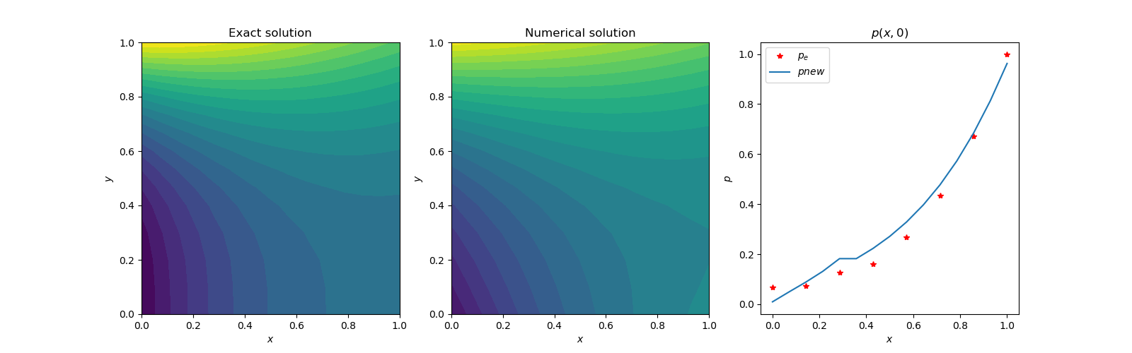 | Figure 4(a). Contour plots of exact and numerical solutions in area A |
 | Figure 4(b). Numerical solution in area A |
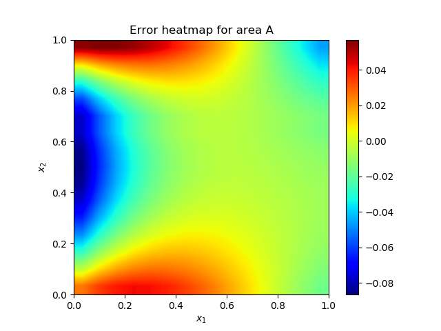 | Figure 4(c). Heatmap of the solution error in area A |
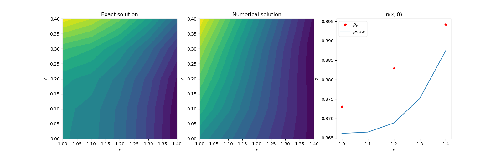 | Figure 4(d). Contour plots of exact and numerical solutions in area B |
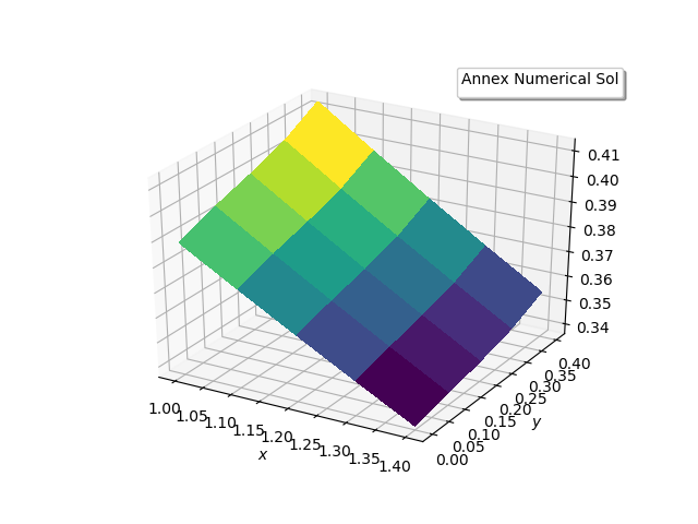 | Figure 4(e). Numerical solutions in area B |
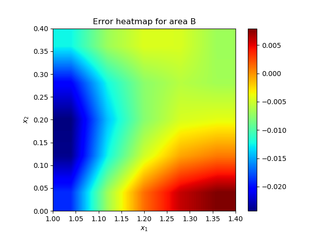 | Figure 4(f). Heatmap of the error in area B |
Another way to solve this problem would be to patch one continuous domain of two-dimensional coordinates. This method does not have any interface. Proper boundary conditions are applied at the boundaries. Only one neural network is required. The results are shown below and are in good agreement with previous method.
3. Conclusions
The present simpler new neural network scheme with explicit boundary conditions exhibits nice capability to solve elliptic partial differential equations Both uniform and random grids can be used in the square or rectangular solution domain. With the correct boundary conditions and source function, solution can even be obtained with modelling error such as omission of Laplace operator itself. The residual errors shown in heatmaps can further be reduced by BFGS-scheme [2]. The complete Python program for this paper can be downloaded from narain42/Poission-s-Equation-Solver-Using-ML on github.com.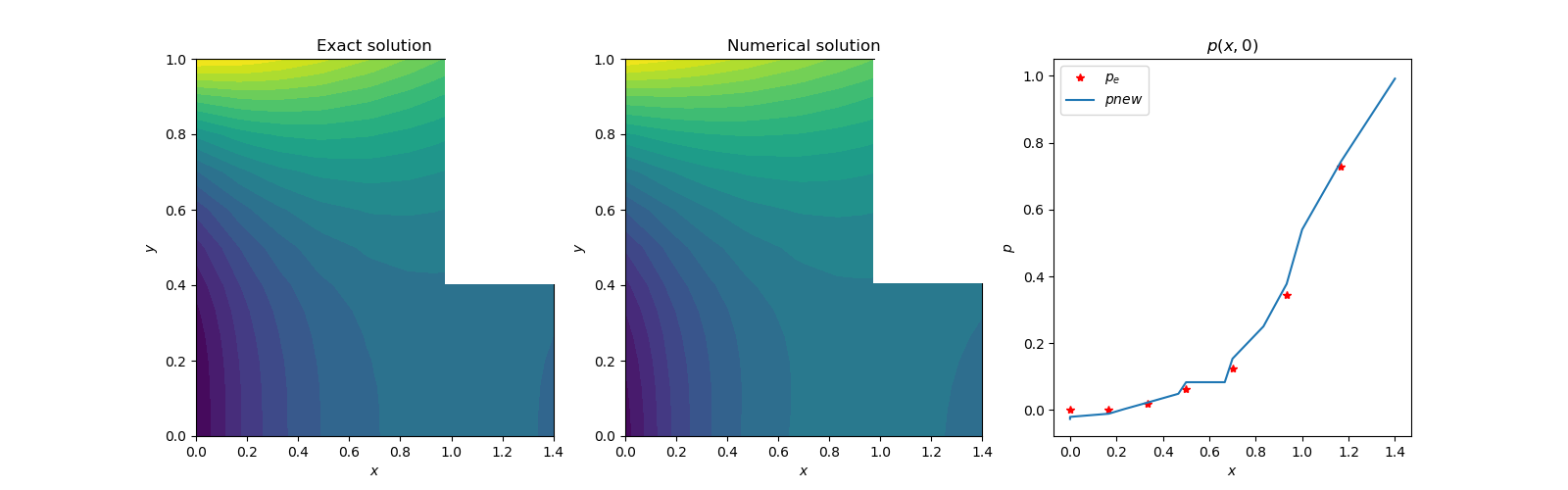 | Figure 5(a). Contour plots of exact and numerical solutions |
 | Figure 5(b). Numerical solutions in the entire domain |
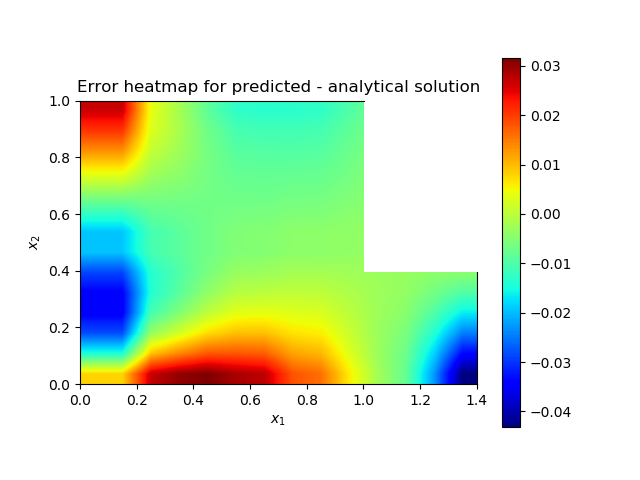 | Figure 5(c). Heatmap of the solution error |
References
| [1] | I.E. Lagaris, A. Likas, and D.I. Fotiadis, “Artificial Neural Networks for solving ordinary and partial differential equations,” arXiv:physics/9705023v1, 19th May 1977. |
| [2] | Lu Lu, “DeepXDE: A Deep Learning Library for Solving Forward and Inverse Differential Equations”, AAAI-MLPS, March 24, 2020. |
| [3] | J.P. Narain, “Solution of Poisson’s Equation Using Artificial Neural Network”, Computer Science and Engineering, Vol. 11, No. 1, June 2021. |
| [4] | Ryan Adams, “autograd”, HIPS/autograd on github.com, March 5, 2015. |
| [5] | Luis, Angel, “Solving differential equations with neural networks,” imyoungmin/DENN on github.com, May 2, 2019. |
| [6] | Findiff library, pypl.org/project/findiff, Feb 12, 2021. |
| [7] | NumPy, “The fundamental package for scientific computing with Python”, numpy.org, 2021. |
| [8] | Diederik P. Kingma, Jimmy Ba, ”Adam: A Method for Stochastic Optimization”, arxiv, 2015. |

 Abstract
 Reference
 Full-Text PDF
 Full-text HTML