1. Introduction

The ordinary and partial differential equations have been solved anaytically and numerically for many years. Various numerical schemes were developed with the advent of computers. From such schemes, the finite difference scheme has been a popular numerical method. Findiff library from PyPl offers a Python package to solve such equations in any number of dimensions [3]. The boundary condition based neural network method for non linear Blasius equation using autogad library [4] was investigated by Kitchin [5]. This work was extended to more complicated Falkar-Skan equations by Narain [6]. The neural network schemes require derivative of neural network. The autograd library [4] was used in these methods for equations in one dimension. The present work is aimed at solving Poisson’s equation in two dimensions. This equation is used in many engineering fields such as fluid dynamics, electrostatics, traffic control system, etc. Angel [2] has developed a nice scheme for multi -dimensional neural network and their derivatives. With this scheme, any ordinary and partial differential equation can be solved with ease. Most of the applications have been for Laplace equation which is Poisson’s equation with no source term. Several examples for Poisson’s equation will be presented together with comparison with finite difference scheme.

2. Discussions

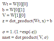
Poisson’s equation is

𝛥𝛟 = f

where 𝛥 is the Laplace operator, and f and 𝛟 are real or complex valued functions on a manifold. Usually, the source function f is given and 𝛟 is sought. When the manifold is Euclidean space, the Laplace operator is often denoted as 𝛻² and so Poisson’s equation is frequently written as

𝛻² 𝛟 = f

In two-dimensional cartesian coordinates, it takes the form

d² 𝛟(x,y)/dx² + d² 𝛟(x,y)/dy² = f(x,y)

when f =0, we obtain Laplace’s equation. cartesian coordinates_.

To solve any equation, boundary conditions are needed. There are three type of boundary conditions (b.c.), for example boundary condition on edge y=0 would be

𝛟(x,0) = a(x)

which is the Dirichlet Boundary condition, and

d 𝛟(x,0)/dn = b(x)

which is Neumann boundary condition. A mixture of Dirichlet and Neumann is termed as mixed boundary condition. dn denoted normal direction on an edge.

There are several ways, this equation can be solved. Exact solution can be obtained using Green's function and other methods. Very fast and accurate numerical solution can be obtained using finite difference, finite volume, finite element and other methods. The matrix inversion methods are efficient for small dimensions, Jacobi and Gauss-Seidel iterative methods are good for any dimension and any boundary condition. The gradient decent and conjugate gradient methods are more efficient but are limited to zero Dirichlet boundary conditions on the edges.

Following ref 2., the neural network for a two-dimensional case is defined as

Define neural_network(x,W) as nnet:

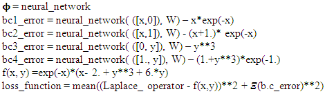
The important neural net derivative function is defined as

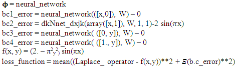
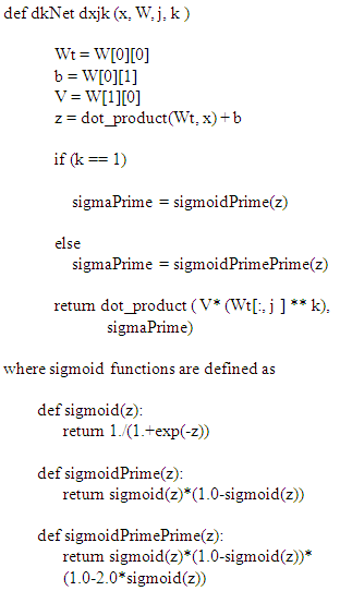Here x is the input vector with two coordinates (x,y), W is the network weight and b is the bias, j denoted direction of partial derivatives (0 for x, 1 for y), and k stands for partial derivative order ((1 for first order, 2 for second order).

The loss function is defined as

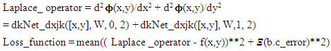Where is the summation indicator for all the boundary condition errors. An example of b.c error will be 𝛟(x,0) - a(x).

Next the gradient of the loss_sum is minimized by Adam scheme [4]. In general, the nnet function is initialized with random numbers. Thus, the initial solution will look totally different from expected solution. After five hundred iterations, the solution converges. The predicted solution matches pretty well with the FinDiff or exact solution.

Next we will examine two cases from ref. 1. One has Dirichlet boundary condition. Other one can be solved both in Dirichlet b.c. mode or as a mixed b.c. mode. We shall use mixed b.c. mode as it will show the ease of problem setup for such case.

The complete Python program for this paper can be downloaded from narain42/Poission-s-Equation-Solver-Using-ML on github.com.

3. Examples

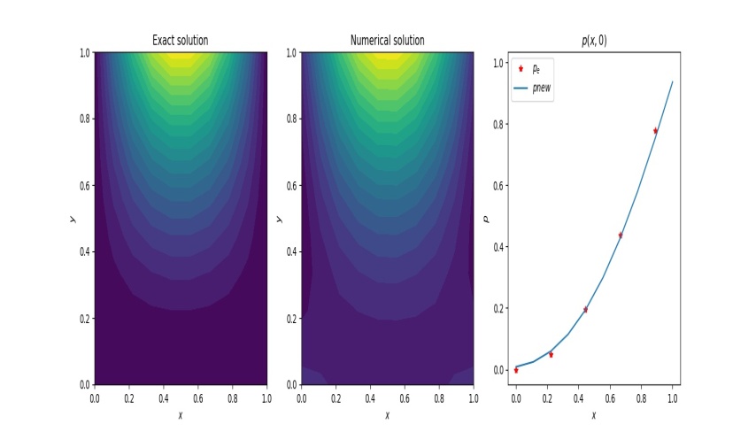
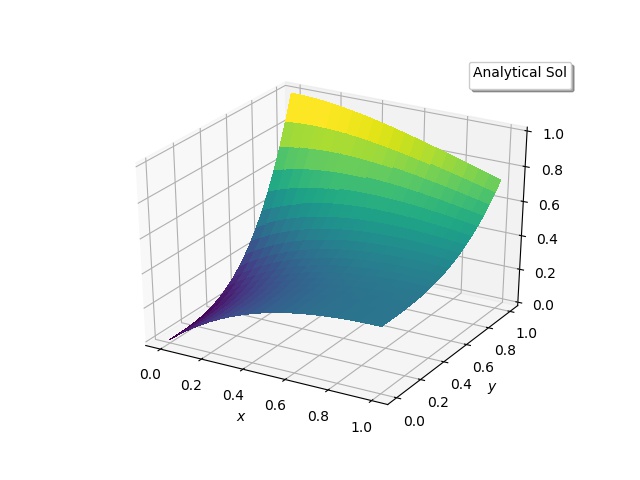
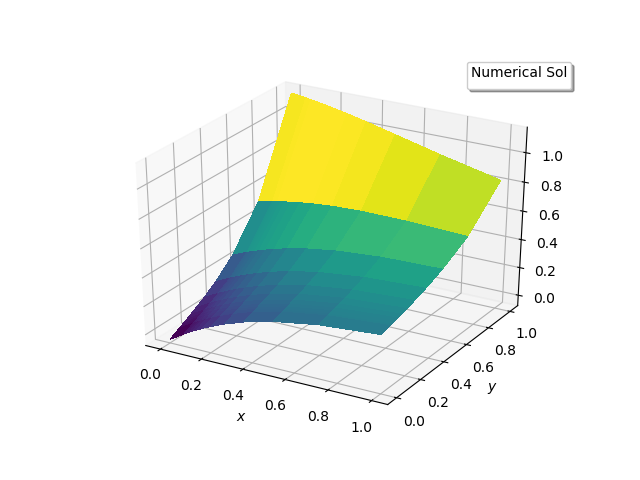
The first example, Problem 7 of ref. 1, is a very simple case with zero Dirichlet b.c. on three edges, and a non-zero either Dirichlet or Neumann b.c. on one edge. The following are the details:

𝛻² 𝛟 (x, y) = (2. – π²_y²) sin(πx)

with x, y ϵ [0,1] and with mixed b.c, 𝛟 (0, y) = 0, 𝛟 (1, y) = 0, 𝛟 (x,0) = 0, and d 𝛟(x, 1)/dy = 2 sin(πx).

First the FinDiff , finite-difference solution is obtained. The solution plots are shown below.

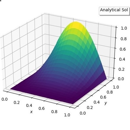Figure 1(a). Exact solution

Figure 1(b). Numerical Solution

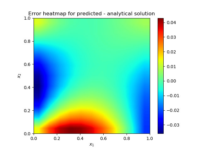
Figure 1(c). Error between solutions

For Artificial Neural network solution [1], the boundary conditions are embedded in the neural network [1]. The suggested trial solution for Neumann b.c is

𝛟_trial(x,y) = B(x,y) + x(1-x)y[N(x,y,p) – N(x,1,p) -d(N(x,1,p))/dy}

Where B(x,y) is related to the b.c, and N(x,y,p) is related to the neural network.

In the scope of present neural network model, differentiating the trial function for Laplace operator will be a complicated task. The simple boundary condition scheme model is as follows

This is all what is required to do the Adam [4] optimization to get the desired solution. The results are:

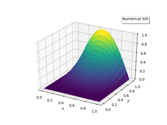
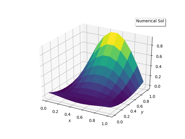Figure 2(a). Numerical solutions

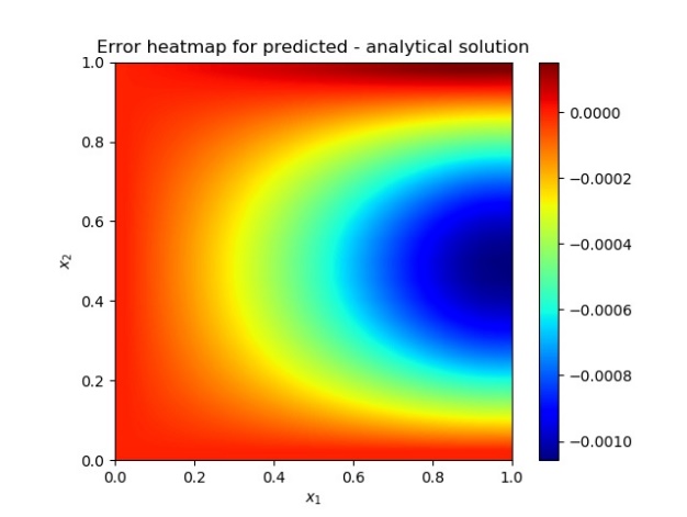
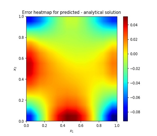Figure 2(b). heatmap of the solution error

Figure 2(c). Contour plots and comparison with exact solution

The FinDiff solver takes less than 2 seconds, while neural network iterations on (21x21) grid domain took around 1760 seconds for 500 iterations.

Next case is problem 5 of ref 1. This has Dirichlet boundary conditions on all edges. The numerical model is as follows:

This model is used in Adam [4] optimization to get the desired solution. The Dirichlet b.c. problems converge faster than Neumann conditions. It took only 580 seconds on a (15x15) grid, with 5000 iterations, to converge. No FinDiff results are presented to save the length of this article. The results are similar to those presented below.

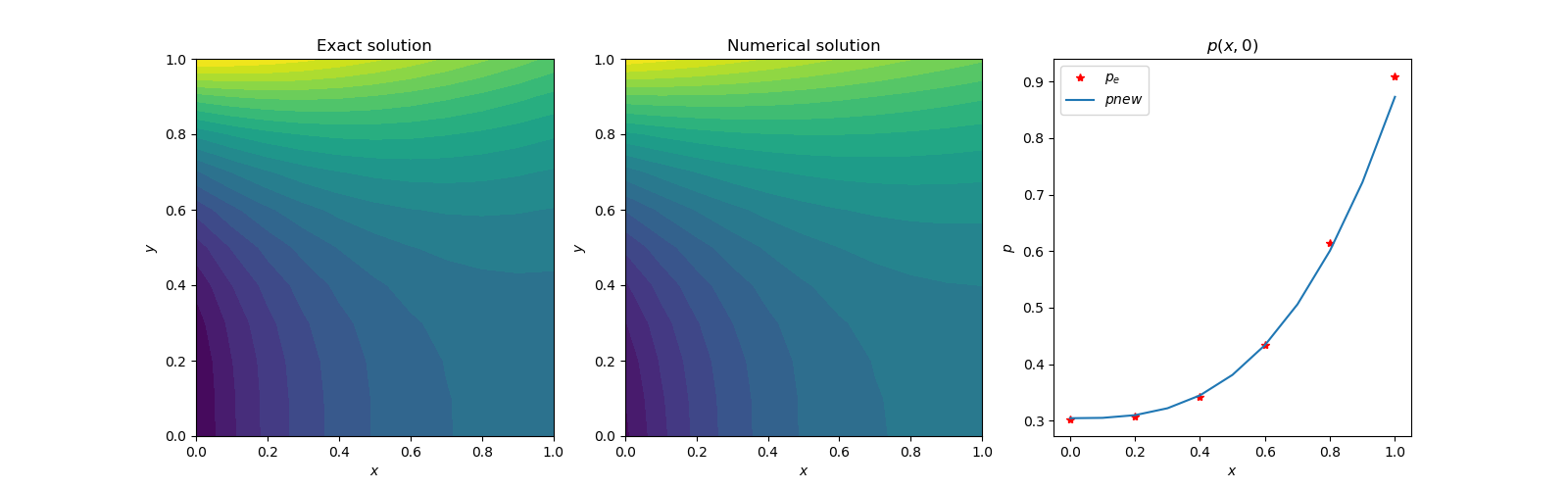Figure 3(a). Contour plots and comparison with exact solution

Figure 3(b). Exact solution

Figure 3(c). Numerical solution

Figure 3(d). Heatmap of the solution error

4. Conclusions

The new neural network scheme seems to be an efficient way to solve partial differential equations up to second order. The method was applied to first order linear and non-linear partial differential equation cases. Although the results are not reported to keep this paper concise, the results were precisely similar to FinDiff solutions.