1. Introduction

The total energy usage in the world is largely covered by building sector consuming about 40% of the electricity usage [1]. Thus, it has become paramount to forecasts building energy usage to reduce high CO₂ emissions and for efficient decisions making. Accurate forecast would assist engineers and architect to explore different design options and strategies for building operations. Recently a lot of attention and effort have move towards the design and implementation of smart buildings to balance the demand and supply of electricity effectively [2].

Consumption of electricity is increasing in the last decade as urban areas are constantly increasing respectively [3]. Hence the growing need to bridge the gap between electricity demand and supply, this can be achieved by improving the forecast accuracy thereby enhances planning [4]. Also a minimal improvement of 1% in prediction accuracy will in turn save millions of pounds each year [5]. Thus, economic reasons are the main motivation behind load prediction [6]. Based on this reasons among others, a number of technique and computational methods have been implored recently to improve the prediction accuracy [7].

According to Mocanu et al. [8], electricity forecasting can be grouped into either one of these three groups: (i) short term forecast usually ranging from day-week (ii) medium term forecast usually ranging from week-year and (iii) long-term forecast usually ranging from year and above. Physical or data driven bases are the main method or approaches that are implored in the context of electricity prediction [1]. Physical approach mainly depends on the physical principles, building details, and its properties to characterized building behaviors; thus, refers to as the white box models. The performance of this model is subject to fluctuation, because it requires large amount of information thus becoming computationally expensive, particularly if the assumption of this information is not completely fulfill since the model capture building response to influential factors including the outdoors and indoors environment [9]. But a major drawback of this deterministic model is not being able to account for complex consumption behaviors and difficulty in obtaining the input parameters required, thus making poor predictions sometime up to 100% lost in accuracy [9]. Although other options to such models is statistical and ML models [9] and have been successfully applied in this context, such as LR [10], SVM [11] Extreme learning machine [12], stochastic model (CRBM and FCRBM) [8], LSTM [13], RNN [14], Elman neural network [15], Deep Recurrent Neural Network [5] and ensemble technique [16]. Physical models can be hybridized with machine learning models to form hybrid models which have also been proposed in the literature, such as the study in Fu [17]; the Hybrid model is an experiential approach decomposition of DBN and assemble system. In general, hybrid models have proof to achieve high accuracy particularly short-term forecast an hour [18] to a week [19]. But there are few limited work pertaining medium to long term prediction with previous work showing errors in excess of 40-50% as regard to medium to long term forecasting [13].

Deep neural networks [5] could greatly improve on the general performance to existing related predictions models by applying multiple layers of abstraction which permit them to model more complex functions [20]. Neural network [21] is popularly applied in electricity load forecasting [22]. The approach tries to learn or model both the input and output nonlinear relationship. Recently, deep learning neural networks [23] have been rapidly develop and have shown to attained higher improvement in prediction as compare to their counterparts’ traditional shallow neural networks. This improvement was achieved due to three reasons which include: a better learning algorithm with multiple hidden layers and the initialization approach of the parameters has greatly contributed towards the success of deep learning approach [24]. Deep recurrent neural network accommodates temporal dependencies of both short and long term as shown by [25]. DRNN address the short comings of long term forecasting observed in previous literature [5]. Despite being a very strong modeler, RNN comes with a shortcoming of training difficulties which was overcome, thereby allowing their smooth application to difficult sequence complications [15].

A number of technique and computational approaches have been implored recently in order to improve the prediction accuracy. These techniques as presented by Rahman et al. [5] would likely have decreased accuracy in application if the weather in the future was significantly different from the weather that was concurrent with the training data. Similarly, there are few limited work pertaining medium to long term prediction with previous work showing errors in excess of 40-50% as regard to medium to long term forecasting [13].

This paper is aimed at designing and implementing a model that predict electricity consumption in residential buildings by enhancing the prediction reliability using NARX with LSTM network while including whether information as an external factor to the prediction and evaluate the results against the state of the art. The key contribution of this study is implementing the NARX-LSTM base Network that addresses the high error associated to medium and long term forecast by curtailing future impact of weather to the prediction results, thus enhancing the accuracy and reliability of the proposed model against state-of-the-art prediction techniques use in energy forecasting. The result from this model will greatly assist Jos electricity distribution center in planning and adjusting electricity demand and supply respectively, based on the authors knowledge, no research work of this nature has been carried out in Jos electricity distribution center. Thus, this research hugely contributes to the community.

The rest of this paper is divided into sub-sections. Section ii details the theoretical background of Deep Learning methods including ANN, DRNN, NARX and the MLP. Section iii presents the formulation and description of the proposed NARX-LSTM model and the scheme for data normalization and further describes the evaluation setup, Section iv analyzed the simulation results and section v concludes by summarizing the key results, while section vi identified the limitations and confers paths for future research.

2. Literature Review and Theoretical Framework

This section presents the theoretical background and historical reviews of deep learning computational technique so as to explore the fundamentals of this research work and also identify the recent state of art prediction techniques use in energy forecasting.

2.1. Artificial Neural Network

ANN is an intelligence computing approach that is made up of neurons which is stirred by the biological neurons. The input and output relationship are complex and is model by activating each neuron from the input node and sends the response to the output node. the traditional ANN is consisting of three main layers (input, hidden and output layers), these layers are interconnected. Each of these layers is comprise of multiple neurons with an activation function with no any systematic framework for selecting the numbers of hidden layers. Although three categories of parameters are implored to define ANN, this includes the connection style, learning procedure and activation [26]. ANN has been applied in different areas because of their intelligence performance such as speech recognition, robotic control, image processing, data mining, and energy forecasting [4]. Trial and error are the most widely method of determining the number of hidden layers for the network training. The error in the network weight is minimized during the training phase, when one of the following occur the training is terminated i.e the gradient performance is below a threshold or the required value is met for the error that is minimized [27]. Despite the computational power of ANN, it comes with a number of draw backs such as model over fitting, random weight optimization sensitivity and probability of local optima convergence. [28].

2.2. Deep Recurrent Neural Network (GRU and LSTM)

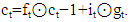
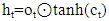
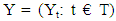
A recurrent neural network can be extended to a deep recurrent neural network via different ways as shown by Pascanu et al. [29]. The concept of depth in RNN was initially argued, but base on the architecture of RNN, three areas can be make deeper in other to construct a DRNN, this includes; hidden to hidden function, hidden to hidden transition and hidden to output function [29]. There are different variants of DRNN but we will focus on the popular DRNN use in the context of electricity forecasting including LSTM and GRU. The idea of RNN_S with gated units was first introduced by Hochreiter and schmidhuber. [30]. LSTM is suitable for modeling long range dependencies, LSTM's architecture has memory blocks Compared to RNN which has hidden units [31]. The memory cells which are modulated by nonlinear sigmoidal gates are contained in a memory block, which are multiplicatively applied. Memory of the same gates share cells so as to reduce the parameters. The model stores the values at the gates (when the gates evaluate to 1) or remove them (when the gates evaluate to 0) as determine by the gates. With this, long-range temporal context can be exploit by the network [32]. In order to solve the problem of vanishing gradient during forward and backward phases, the vanishing gradient are alleviated to allow the network preserve it memory over some time steps. The studies in Chung et al. [33], found both GRU and LSTM to be comparable. Training speed of GRU is faster due to the less parameter as compared to other RNNs such as vanilla RNN [34].

An LSTM layer is a Recurrent Neural Network (RNN) layer that enables support for time series and sequence data in a network. The layer performs additive interactions, which can help improve gradient flow over long sequences during training. The LSTM Layer Architecture use in this work is depicted in fig 1. The diagram demonstrates the flow of a time series X with D features of length S through an LSTM layer. Where h represents the output (hidden state) and c represents the cell state. The first LSTM unit takes the initial network state and time step of the series X1, and then calculates the first output h1 and the restructured cell state c1.

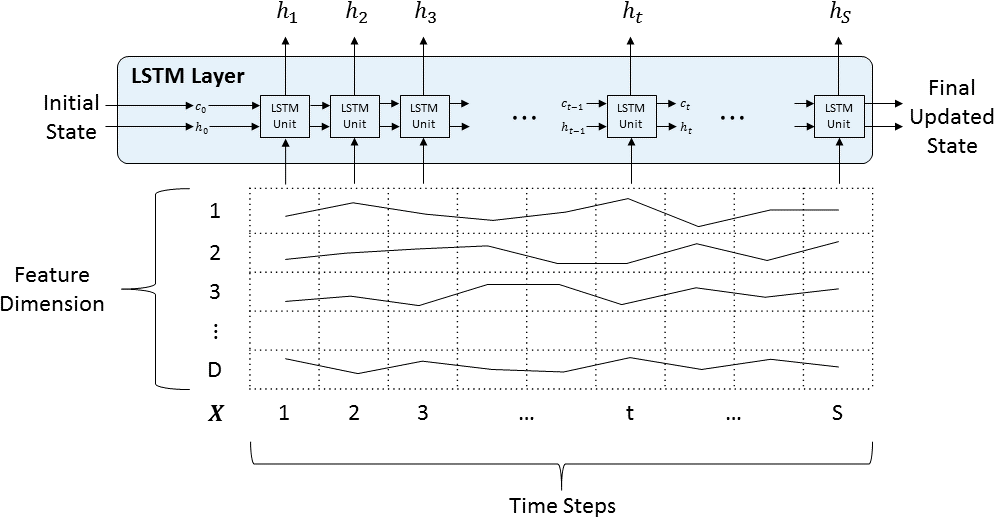Figure 1. Architecture of LSTM layer Hochreiter and schmidhuber [30]

At time step t, the unit takes the network current state (c_t−1,h_t−1) and the resulting time step of the sequence X_t, and then calculates the output h_t and the updated cell state c_t [30].

at given time step t, the cell state is computes by:

(1)

where ⊙ represents the Hadamard product.

The output also known as hidden state at time step t is computed by:

(2)

The learnable weights of an LSTM layer are the input weights W, recurrent weights R, and bias b which is concatenated as presented in the following matrices. input weights W= [W_i W_f W_g W_o], Recurrent weight R= [R_i R_f R_g R_o] and bias of the respective component b= [b_i b_f b_g b_o]. where f, g, i, and o represent the forget gate, layer input, input gate, and output gate, respectively [30].

2.3. Nonlinear Autoregressive Neural Network (NARX)

The NARX network is a recurrent dynamic network, with feedback connections enclosing several layers of the network making it suitable for time series forecasting. Time series are a sequence of data, numerical values or observations usually recorded at constant time intervals [35]. It is measured normally every second, minute, hour, day and week or in some cases year. A time series connecting to the variable Z over the time set T is denoted by

(3)

In which, Y_t is the value of Y at time T. the energy consumption of a building for example, defines a time series, showing in each instant the consumption usage of the building. In many cases, this data depends not only on the total amount of usage but also on different other possible influential factors. NARX neural networks have demonstrate to tackle this factors which is very helpful tool in time series environments [36]. These models are a kind of recurrent system which improved the approximation of the ANN thus reducing the output error with self-learning. NAR make use of past values for the real time series to forecast next values as determined by the equation [4] below [37].

(4)

Where h is a nonlinear function depending on p which is the past values of the output X. NARX has an input and a feedback delay for the input and feedback network and a feedback loop from the network output to the hidden layer.

2.4. Multilayered Perceptron

Multilayered perceptron’s (MLPs) are special form of feed-forward networks also known as universal approximates. MLPs are the most commonly used neural network architectures due to its simplicity [38]. A feed forward network (MLP) has a layered structure, where each layer is consisting of units that receive their input from units from a directly connected layer below and transmit their output to units in a layer directly above the unit. There exist multiple units in each layer and units of the neighboring layers are fully connected to each other, but no connections in the same layer. For a two-layer neural network, this is also known as multi-layer perceptron.

2.5. Convolutional Neural Network

LeCun firstly proposed Convolution neural networks (CNNs) for image processing, where two main properties are featured i.e. spatially spatial pooling and shared weights. CNNs where widely applied in various computer application successfully including sequential data, processing of natural language, speech recognition and image classification. Convolutional Neural Networks mainly focus in learning features that are abstract; this is accomplished via stacking and alternating pooling layers and convolution layers respectively. this convolutional kernels i.e. convolution layers in CNN convolve raw input data with numerous local filters hence yield transform local feature with the succeeding pooling layers’ excerpt features and a static-length of the raw input information in stages of numerous rules such as average and max [39].

The review understood in this section of the research permits the authors to offer the theoretical foundation essential for the improvement of energy forecasting model, which is presented in the subsequent part of this work.

2.6. Related Work

There are three categories and method applied in the prediction of energy usage in building, these include statistical method (black box models), engineering methods (white box models) and hybrid methods (grey box model) [40]. both machine learning and statistical model been employed in the previous works as discuss in the literature. For example, Robinson et al. [41] proposes a machine learning approach using natural data from CBECS to forecast both electricity, fuel, and natural gas consumption of commercial building with the aid of the building features that are accessible, similarly Deng, Fannon, and Eckelman [10] test various predictions models for HVAC and energy usage, an improved accuracy was demonstrated by SVM. Also in the work of Kaur and sachin [42], auto regressive moving average ARIMA was use to forecast electricity consumption. Previously in the context of building energy consumption modeling, machine learning models performs better than linear models for example Tso and Yau [43] test linear regression models decision tree and neural network for electricity consumption modeling at building level in Hong Kong. Similarly, Dehalwar et al. [44] use ANN and bagged regression tree for load prediction using data from the metrological agencies, in both cases, neural network performs better. One of the common limitations among statistical, engineering and hybrid models is the availability of vital data [41].

There have been limited number of work with regard to medium and long term forecasting either sub-hourly or hourly-intervals with long term prediction being more difficult and complex task to achieve, a relative error often in excess of 40-50% is associated with medium to long term forecasting [8]. Potential improvement on prediction accuracy of the aforementioned machine learning can be obtained using deep neural network where modeling of more complex functioning is allowed by the use of several layers of abstraction (24). These approaches are applied recently in the context of energy prediction for example [17] employ deep learning approach for the determination of cooling load prediction which outperforms SVM and BPNN in terms of accuracy and stability. Similarly, Cheng fan et al. [45] Propose a deep learning for building profile load predictions, an enhance performance was obtaining especially when the deep neural network is use in an unsupervised manner. It was also shown in the studies of [8] where the forecasting accuracy was greatly improved by the integration of DBN into a reinforcement algorithm that can target features of the buildings.

The nature of electricity usage behavior is transient, long term dependencies can shape the consumption pattern, one family of algorithm in which the dependencies between consecutive times steps is being accommodate is the recurrent neural network and has been implored in the context of energy forecasting [5]. Recurrent neural networks are known to improve time series prediction errors as shown by (Abdul et al 2018). (Ruiz et al 2017) [46], propose an ENN and optimize the weight with GA, an improved result was obtained compare to previous studies. Similarly, [14] proposed a new recurrent ANN model base on multiplicative neuron model and it was observed that the model produce the most forecast accuracy compared to other forecasting method. However, despite the improvement in the results obtain by modeling time series problems using recurrent neural network, it still suffers from the problem of vanishing gradient as described by hochrieter and Schmidhuber [30] because RNN do not account for long term dependencies. One of the possible solutions to the vanishing gradient as suggested by hochrieter and schmidhuber is RNN_S with long short term memories. [18] use a long short term memory base network algorithm for the forecasting of electricity and compared it to BPNN, MLFFNN where LSTM demonstrate higher accuracy as compare to the aforementioned competitive Algorithm [5] develop two deep recurrent neural networks by Stacking LSTM on top of the model using encoder – decoder design for forecasting of electricity consumption in residential and commercial buildings. The two deep RNN performed better than the MLP.

3. Methodology

3.1. Data Collection and Model Input

To train the model for forecasting, the developed NARX-LSTM network relies heavily on input vectors. Choosing an input vector comprising of external factor produces a better, robust and reliable performance. The proposed model was tested and evaluated on electricity consumption data obtained from the private residentials buildings in Rikkos, Jos City using Smart Software Tools from residential smart meters. The area is located at 9°55’N 8°54’E and mostly covered by residentials buildings of extended families. The dataset that was obtained contains electricity data for 34 buildings for the period 1st January, 2014 to 31st December, 2016. The overall hourly electricity consumption data in residential Buildings can be obtained from Jos Electricity Distribution Centre JED. The features of the dataset consisted of a combination of weather, date and electric load consumption related variables respectively. This electricity consumption data in residential buildings is then aggregated over an increasing number of residential buildings, up to a maximum of thirty-four buildings. For a given number of buildings over which the residential building energy consumption was aggregated, the residential buildings were selected in ascending order of the building ID. The weather data that was used for concurrent training and prediction by the model which was obtained from NCRS-Jos.

3.2. Model System Development

To implement the model, the proposed framework is described below so that the architecture must be able to process the data with a high throughput and accuracy. The architecture of the proposed framework is shown in Fig. 2.

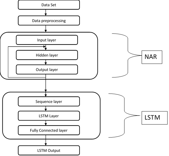Figure 2. Proposed Frameworks

The framework consists of three main stages

Stage 1: Data set Collection and Preprocessing Stage

This stage combines the Data set identification, collection and Preprocessing of the Dataset to remove inconsistencies.

The Data set collection stage involves the identification of predictor variables and Data collection stage. In this experiment, the relevant predictor variables that are significant for the modeling of the system are identified and then selected. After identification of the relevant input variables, the Data set is collected from the official sources and saved in the appropriate data format (.xlsx). The dataset is pre-processed by carrying out data cleaning and shrubbing to eliminate typographical errors and inconsistencies in the data and saved in the format required by Matlab through data formatting phase. We carry out data normalization scheme using the minmax (-1 to 1) to normalize the dataset for fast convergence.

Stage 2: Nonlinear Autoregressive Network with External Inputs Stage

The NARX stage is the stage built on the Sequence Layer of the LSTM Stage. The NARX Stage comprises of Input, hidden and output Layer. The Input and feedback inputs are fed via an input and feedback delays. Fig. 3 shows the NARX Network used in this research. The NARX network used in this research work is designed to accept two inputs which is the electricity data and weather data to be used for the network training concurrently.

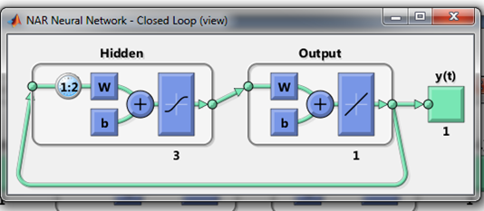Figure 3. NAR Neural Network Closed Loop View

Stage 3: LSTM Stage

The output from the previous NARX stage is fed to the subsequent LSTM stage as input. Sequence input and LSTM layers are the main components in the LSTM stage. The network begins with the sequence input layer followed by a completely connected layer and ends with LSTM output.

The next layer is the LSTM Layer which is the intermediate layer in a LSTM Recurrent Neural Network. long-term dependencies between sequence data time steps is learn by this layer which result to the inclusion of the layer during the design. The LSTM layer also perform additional interactions to models the sequence data of the time series in the network. this help greatly in improving the flow of the gradient in training over lengthy sequences. In order to identify the larger patterns in the data set and make the forecast. The fully connected layer is configured next to combine all the features learned from the previous layers (sequence and LSTM) and Hence, the output size parameter in the last fully connected layer is equated to the number of classes in the target data and a bias vector is added by the fully-connected layer which then multiplies the input by a weight matrix.

The final layer (LSTM output) or (Regression Output) grasps the loss function for regression and response used for training the network.

3.3. Choice of Metrics

For developing forecasting model, the real data is vital. Performance measures allow the evaluation of the accuracy of various forecasting techniques useful to a particular time series. To evaluate the forecast errors, it is necessary to analyzed the performance. Testing the Neural Network is a vital step in the design process. In this experiment, to evaluate the network performance, the Statistical estimating metric presented below is used to ascertain the best performing model. They include: Root Mean Square Error (RMSE), Mean Square Error (MSE), Mean Average Percentage Error (MAPE) and the correlation Error (R).

The Root mean squared error metrics used to evaluate the performance of the models is computed as:

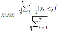(5)

Where, y_a, and y_p represent the actual training and test values for the consumption of electricity respectively.

3.4. Evaluation Setup

The dataset used to train the proposed model contains data for 34 buildings for the period 1st January, 2014 to 31st December, 2016. To evaluate the performance of the models in this study, the data at 30-minute intervals was partitioned into training, testing and a validation set. The features of the dataset consisted of weather, date and electric load consumption related variables respectively. The dataset is Partition into training, test and validation. The first 70% is for training, 15% for test and last 15% for validate respectively.

During the experiment, after importing the data, the input and target data where equated and assigned variables and subsequently transpose from columns to rows. The concurrent vectors are converted to sequential vectors. In order to create the NARX network, the delay of the feedback is set to 1:2; with 3 hidden Layer Size, 2 network Input delay and The Training algorithm is set to Bayesian regularization Back Propagation Algorithm. the data was normalized to scaling [-1 to 1] for the experiment. The NARX network predicts y(t+1) at the same time it is given y(t+1).

The LSTM network in this experiment learns to predict the value of the next time step. For a better fit and to prevent the training from diverging, we standardize the training data to have zero mean and unit variance. In order to configure the LSTM regression network, we specify the LSTM layer to have 200 hidden units. We set the Input Size to be 1 and number of Responses and Hidden Units to 1 and 300 respectively. The LSTM used in this experiment, is comprised of four layers including sequence Input Layer, LSTM Layer, fully Connected Layer and a regression Layer. For options of the training, we set the solver to 'adam' and train for 500 epochs. To prevent the gradients from exploding, the gradient threshold set to 1 and Specify the initial learn rate 0.005, and drop the learn rate after 125 epochs by multiplying by a factor of 0.2. The training progress plot reports the root-mean-square error (RMSE) and compared the forecasted values with the test data.

4. Results and Discussion

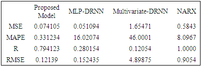
The accuracy of the estimated forecasts of the proposed model was compared with the other models to determine which model gives a more accurate forecast through the use of RMSE, MSE, MAPE Regression or correlation error (R). We will now present the result for the forecasting using all the different algorithms by the performance standard achieved by each of the model and discuss the findings.

The main purpose of the graphs obtained from the model is not to be analysed directly, but rather portrays to the reader a synopsis of the way the trend continues. In order to validate the proposed network, the error autocorrelation is used. auto-correlation analysis provides the basis for immediate future predictions. Fig. 4 display the error autocorrelation function. The figure shows how the prediction errors are related in time. Ideally, for perfect prediction model, there should be only one nonzero value of the autocorrelation function. These nonzero values should occur at zero lag; this is also called mean square error. Such an autocorrelation function would imply complete un-correlation of predicted errors with each other. Base on Fig 4, the correlations, excluding the zero lag, fall almost around the 95% confidence limits within zero, thus the model appears to be suitable. If there were significant correlation in the prediction errors, then it’s possible to improve and enhance the prediction accuracy maybe by changing the neural network structure or increasing the number of delays in the network.

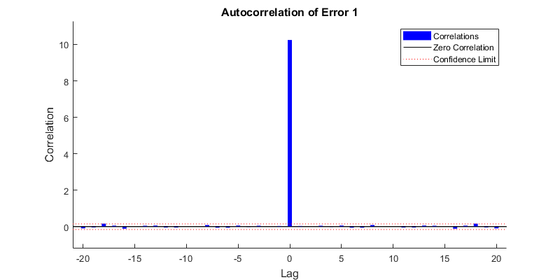Figure 4. Auto correlation error for the proposed model

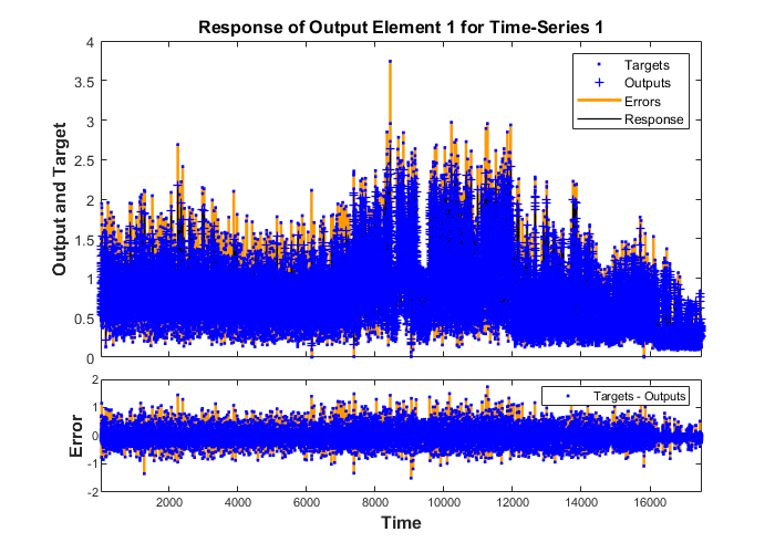Figure 5. Training response for the proposed model

Similarly, Fig. 6 Shows the Error histogram of the fit set for the proposed model.

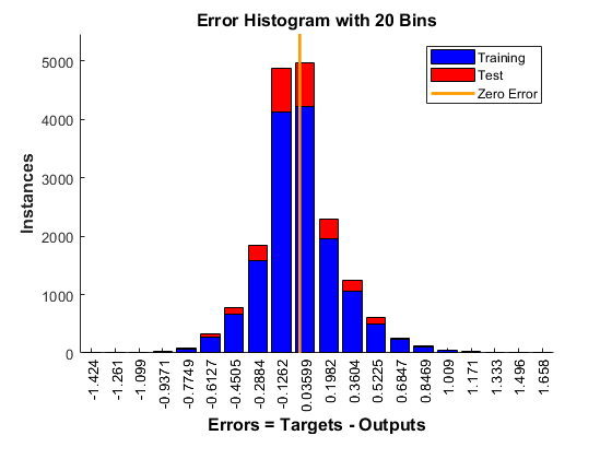Figure 6. Error Histogram for fit set of the proposed model

Fig. 7 shows the regression graph for the proposed model; this shows how accurately our trained model fits the dataset. It was observed that the value of R is close to 1 which imply good prediction which shows that the model prediction is very close to the test dataset. If it was close to zero which imply bad prediction which shows that the model completely fails in making a correct prediction. In our own case, the model prediction was close to the actual test which demonstrate a good prediction by the proposed model as shown in table 1.

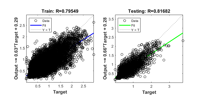Figure 7. Error regression on forecast vs. actual for the proposed model

Table 1. Illustrates how the performances of the proposed deep RNN models compare with those of the MLP model

The proposed model achieved best training performance with MSE of 0.074205 at epoch 208 which was slightly lower to the existing model which have MSE of 0.051094, but the proposed model outperformed all the other models in terms of RMSE, MAPE and correlation error (R). although both models demonstrate some level of accuracy in terms of predicting electricity consumption the existing model outperformed the proposed model in terms of running time (speed) of the algorithm as well, thus becoming a costly limitation and major drawback of the proposed model as against the existing model.

The results in table 2 further demonstrate how the proposed model fit the data as compare to the MLP-LSTM network, NARX network and conventional multivariate LSTM. The proposed model obtains a regression value close to 1 which clearly interpret that the proposed model was perfectly fit for the data used in both the training, testing and validation phase respectively. In order to compare the forecast accuracy using the performance metric, Fig. 8 present all the results obtain base on MSE, RMSE, MAPE and R value.

Table 2. Shows the regression values for the training, testing and validation

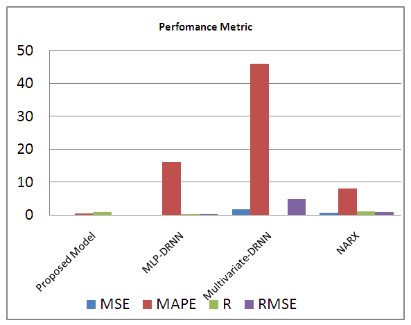Figure 8. Comparison of performance metric use to ascertain the model accuracy

Clearly, from Fig 8. The propose model in general perform better than all the existing models achieving a lower value in terms of MSE, RMSE and MAPE. Moreover, the proposed model combines the weather information and predict concurrently with the electricity data. Thus, the technique has significantly increased the prediction accuracy and reliability by curtailing future alterations of external factors such as the weather uncertainties to the predictions results. As stated earlier, the proposed model suffers in terms of training performance and running cost as against the existing models thus becoming a major limitation of this research work.

5. Conclusions

Recently a lot of attention and effort have move towards the design and implementation of smarter grids in building in order to balance the demand and supply of electricity effectively. A minimal improved of 1% in prediction accuracy will in turn save millions of pounds each year. To curtail the gap between demand and supply, new paradigms have to be employed that will use automated methods to dynamically forecast the buildings energy consumption. Many influencing factors make the prediction complex including: occupancy behaviors, weather conditions, parameter and model selection, missing data or incomplete information, and computation complexity of some models. Physics base or data driven base are the main method or approaches that is implored in the context of electricity prediction. Neural networks are recently applied for solving load forecasting due to their wide application. Deep neural network models provide a practical approach to energy consumption prediction. In this paper, we proposed NARX base deep recurrent neural network model to forecast electricity consumption in residential buildings. The predictions were made in sequences of 24-h at sub-hour resolution over a medium-term time horizon (>1 week). Overall, the proposed neural network models presented in this analysis perform better in forecasting electricity consumption for medium term time horizon. The following conclusions result from this analysis:

• The proposed Deep recurrent neural network model, in general, performs better in terms of validation RMSE, MAPE and correlation error (R) than the existing model in the case of electricity consumption forecasting in residential buildings. The proposed model was able to account for long-term dependencies in the context of electricity consumption. in terms correlation error, the proposed model obtains a regression value close to 1 which clearly interpret that our model was perfectly fit for the data used in both the training, testing and validation phase respectively.

• The proposed model uses external inputs (weather information) to forecast concurrently in other to curtail the uncertainty of weather condition which make the prediction more reliable and robust to future weather fluctuation.

6. Limitation

The major limitation of the proposed model is that the model might probably yield inaccurate results when forecasting electricity consumption for dissimilar buildings or even for the identical buildings if major modifications have been made to its structure, equipment, occupancy or operations. Thus, the model couldn’t capture the influence of occupancy behavior and other future alterations to the prediction model. In our future work, this will be included.

ACKNOWLEDGEMENTS

This study was supported by the Tertiary Education Trust Fund (TETFund) Institutional Based Research (IBR) Fund, through the directorate of Research and Innovation of Abubakar Tafawa Balewa University, Bauchi.