Marcelo Flores1, Cabral Lima2, Antonio Thomé3, Adriano Cruz4, Adriana Soares5
1Schlumberger Brazil - Federal University of Rio de Janeiro UFRJ, Rio de Janeiro, Brazil
2Computer Science Department, Federal University of Rio de Janeiro UFRJ, Rio de Janeiro, Brazil
3Computer Science Department, Federal University of Rio Grande do Norte UFRN, Natal, Brazil
4Electronic Computing Institute, Federal University of Rio de Janeiro UFRJ, Rio de Janeiro, Brazil
5Psychology Department, Postgraduate Program, Salgado de Oliveira University UNIVERSO, Niterói, Brazil
Correspondence to: Cabral Lima, Computer Science Department, Federal University of Rio de Janeiro UFRJ, Rio de Janeiro, Brazil.
| Email: |  |
Copyright © 2015 Scientific & Academic Publishing. All Rights Reserved.
Abstract
Fluid level monitoring is an important control process in engineering systems. The level measurement of fluids having changeable densities is a complex task. Most measurement methodologies use sensors that are periodically paused for recalibrations. For flammable liquids, this may be unsafe and even dangerous. This paper proposes a safe recalibrating-free computer-based methodology for measurement of fluid levels, which is based on Hough transform, image processing and normalization. This paper also describes experiments using a prototype of a distillation unit that was built especially to test the proposed methodology. The results from these experiments have demonstrated robustness, low-cost and suitability of the methodology for real crude oil level measurement in distillation processes.
Keywords:
Liquid level measurement, Hough transform algorithms, Canny detector, Visual monitoring normalization, Image processing
Cite this paper: Marcelo Flores, Cabral Lima, Antonio Thomé, Adriano Cruz, Adriana Soares, Measuring Fluid Level through a Recalibrating-Free Hough Transform Methodology, Computer Science and Engineering, Vol. 5 No. 3, 2015, pp. 47-58. doi: 10.5923/j.computer.20150503.01.
1. Introduction
Several engineering processes require fluid level measurement for controlling purposes. These measurement activities frequently use sensors and follow a beforehand methodology. In this context, “methodology” means the clustering of computer processes, methods, algorithms and practical tools that (together and under special rules) monitors the dynamic level of a fluid. In level measurement an applied methodology is classified as intrusive (contact) or nonintrusive (noncontact). Intrusive methodologies have the sensors in a quite continuous contact with the liquid and therefore they are not suitable for dangerous environments. In nonintrusive methodologies there are no (or a very little) contact with the liquid during the level monitoring. Although traditional sensors, such as floats and infrared, are hitherto the most used practical tools for level measurement, they are not recommended for monitoring processes of flammable fluids or even fluids having unstable characteristics (such as density and color). Floats are almost useless for measuring fluids that modify easily their densities or viscosities. Infrared sensors, although more accurate than floats, have not been widely used in flammable liquid level measurements. In crude oil distillation monitoring, for instance, from which are derived diverse fractions of oils with different densities, infrared sensors are rarely applied due to their inadequacy for following dynamic changes. Indeed, from a crude oil sample it is possible to derive (according to their boiling points) several products with different viscosities, densities, colors etc.A variety of acoustic and optical sensors is used in noncontact methodologies. Acoustic sensors usually apply ultrasound techniques. They run by emitting short pulses in the direction of the liquid surface and then measuring their back reflections. These sensors are very sensitive to temperature fluctuations, which are able to change the speed of the emitted sound. They also are very sensitive to the environment circumstances and the presence of some gas can attenuate the ultrasound pulses [1]. An optical sensor measures the quantity of light and translates it into a readable form. A number of optical noncontact sensors have been specially developed for level monitoring purposes [2], [3]. Nevertheless optical sensors require calibrations during the monitoring process in which a series of measurements and human interventions must be applied. Indeed, most of the methodologies currently used for fluid level measurements have parameters that need recalibrations during the monitoring process. This frequently requires to pause the measurement activities, to take into account the new fluid characteristics, to reset sensor parameters, and then to resume the process. All this kind of tasks requires human interventions that must obey a standardized methodology. This kind of methodology is generally beforehand conceived and its success usually depends on the accuracy of the human interventions during the process. Therefore this kind of methodology is not recommended for level monitoring processes of crude oil distillations, for instance, since crude oil is a dangerous liquid whose level measurement activities cannot be stopped without increasing risks to the whole level monitoring process.This paper presents a computer-based methodology for liquid level measurement. VILEMEM (VIsual LEvel MEasurement Methodology) is a novel methodology enclosing a set of new algorithms, methods, processes and practical tools, aiming to monitor liquid level measurement activities. The main contributions of VILEMEM are low-cost, fluid-density independence, non-contact approach and recalibrating-free methodology. It uses Hough transform, Canny detector, visual normalizations and enhanced image processing techniques [4-8]. This paper also presents DUVE (Distillation Unit for VILEMEM Experiments), a simple fractional distillation unit specially built to test VILEMEM through several experiments using crude oil samples. The results of these experiments have shown that VILEMEM can be successfully applied in industrial crude oil level measurement activities.The remainder of this paper is organized as follows. Section 2 presents a review of the principal concepts and methods used in the subsequent sections; describes the simplified distillation unit DUVE, the level measurement module (LMM) and its processes and algorithms to correct image distortions, to identify bottom and lateral edges and to detect current level. Section 3 introduces new algorithms to obtain level measurements based on identification of edges and image normalization techniques, and describes the proposed VILEMEM Algorithm. Section 4 shows the main obtained results of the experimentation of VILEMEN methodology with a lot of experiments with crude oil samples. Section 5 discusses the merits of the proposed methodology and presents the conclusions of this paper.
2. Crude Oil Distillation Processes
Crude oil is composed of aliphatic hydrocarbons. The length of an aliphatic compound depends on the quantity and configuration (chain) of carbon atoms. Diverse products may be derived from the crude oil and the main difference among them is the length of their carbon chains. The longer the chain is the heavier the product is. For instance, gas has few carbon atoms, such as methane CH4, ethane C2H6, propane C3H8 and butane C4H10, that boil at -258.7oF, -127.5oF, -43.8oF and 31oF, respectively. Light naphtha has chains from C5 to C6 and boiling points from 86oF to 194oF. Heavy naphtha has chains from C6 to C12 and boiling points from 194oF to 392oF. Liquids from C7H16 to C11H24 (such as gasoline) have their boiling point from 100oF to 400oF. Chains from C12 to C15 (such as kerosene) have their boiling from 302oF to 572oF. Chains from C11 to C19 (such as diesel fuel, lubricating oils and heavier fuel for heating houses) have their boiling points from 392oF to 662oF. Solids over C19 are the heaviest derived products (such as paraffin wax, tar and asphaltic bitumen) and have the highest boiling points (around 977oF). Crude oil is universally classified as extra heavy, heavy, medium, light, and extra light. Each one of these classes has its variety and quantity of derivable products. The widely used way to determine the brand and the quantity of products derived from a crude oil sample is through a fractional oil distillation unit in which the products are separated by their boiling points. The information gathered from a distillation is important to determine the quality of the crude oil (that implies the cost of refinement), an essential premise for guiding investment decisions which influence petroleum market prices. The extra light type is easier and cheaper to refine than the others and consequently its market price is higher. Inversely, the extra heavy is less valuable because of its cost of refinement. In [9] some interesting fundaments about crude oil distillation processes are shown. [10] describes a mathematical model for fractional distillations. [11] shows a thermodynamic analysis of crude oil distillation systems.
2.1. The Distillation Unit DUVE
A simple crude oil distillation unit like DUVE includes several parts such as a boiler, a distillation column, a top condenser, a lateral condenser and a conveyor belt with a set of collecting devices as showed in Figure 1. Once the different sub products that come up from a crude oil sample melt at different boiling points, the system gathers each fraction in different collecting devices in order to provide a way to analyze its volume and quality.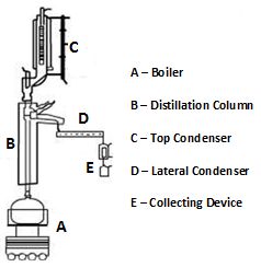 | Figure 1. Main parts of a simple oil distillation unit |
Whenever the capacity of the collecting device is reached ( ) or the current sub product has been wholly melted, the conveyor belt is activated positioning the next collecting device below the spout. DUVE is a simple prototype of a distillation unit specially built for the conception and construction of the visual system research in an academic laboratory. It includes a special collecting device as shown in Figure 2, a distillation column, a suspended reservoir for the oil fraction and a manual system to control the oil flow. DUVE uses a translucent collecting device in order to facilitate the visual measurements and the device has three distinct regions: a top region (the neck area), a false bottom region and a measurable region (the cylindrical middle area). The top and the false bottom regions do not gather liquids. The false bottom holds a digital barcode that is read by the visual system in order to identify and connect each collecting device with its respective oil fraction.
2.2. The Level Measurement Module
A fluid level measurement methodology is classified as contact or non-contact according to the need (and amount) of manipulations required during the measurement activities. When a methodology assists all the steps of the whole measurement activity it is classified as global, and local otherwise. VILEMEM is a synchronous non-contact and global measurement methodology. VILEMEM encloses a Programmable Logic Controller (PLC), a Supervisor System and a Visual Monitoring System. The PLC is responsible for dealing with all signals sent by the sensors and for redirecting them to the Supervisor System. The Visual Monitoring System is the part of the sensor array that is interconnected to the PLC through a field-bus network. The electric signals interchanged between the Supervisor System and the Visual Monitoring System is done through the PLC, and a specialized tension adapter circuit matches the voltages varying from five to twenty-four volts. The Visual Monitoring System has two main modules, the First Drop Fall Detection and the Level Measurement Module (LMM).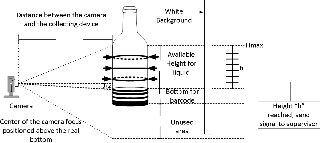 | Figure 2. Regions of a collecting device |
Before the LMM can be activated (at the beginning of a measurement activity) the following human interventions are required just to start the distillation environment: i. put the collecting devices on the conveyor belt; ii. place the camera and calibrate its active angle; iii. verify the position of the lighting apparatus; and iv. hang up a white screen. For simplicity it is assumed that the distillation maintains a steady behavior, such as the liquid never slipping through an edge of the collecting device. The camera is rotated  clockwise to improve the visualization and to capture the largest side of the collecting device. Firstly, the camera and the artificial illumination are turned on by a signal from the Visual Module System, after that the Supervisor System is notified and then verifies the position of the current collecting device. The First Drop Fall Detection module detects the fall of the first drop and the LMM is activated.The LMM finds the false-bottom region, identifies both the barcode and the measurable cylindrical region. The camera begins capturing frames that are put into a FIFO list. The level measurement starts and whenever the current product increases the level of a
  , the LMM sends a signal to the Supervisor System, and the current volume is immediately calculated. When the level reaches the
  (or there is no more liquid to be extracted under the current temperature) the LMM is notified and is automatically paused by the Supervisor System while the collecting device is replaced. When this task is over, the Visual Module System notifies the Supervisor System that verifies whether the new collecting device is placed and then the measurement activity restarts. The LMM carries out five main processes: i. correction of image distortions; ii. barcode detection and interpretation; iii. identification of the lateral edges; iv. identification of the bottom; and v. detection of the current liquid level. Figure 3 shows a block diagram of the main monitoring activities.
 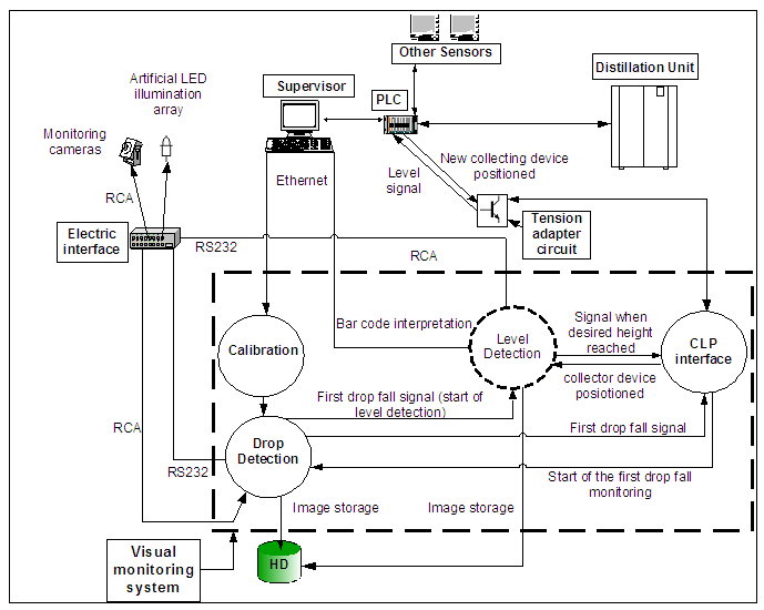 | Figure 3. Main monitoring activities |
2.3. The LMM Correction of Image Distortions
All images are susceptible to geometric distortions caused by variations in camera lens. These come from variations of the image magnitude and its distance from the focal axis. The sources of these distortions (and lens positioning errors) vary according to the configuration, however it is vital to remove (or at least to reduce) these distortions before gathering measurements. The best-known distortions are the cushion form and the barrel form [12].A cushion form distortion enlarges as the distance from the center increases, whereas in a barrel form distortion the magnitude decreases as a function of the distance to the center of the image. A digital camera with a wide-angle lens, such as the one used in DUVE, causes a barrel form distortion (Figure 4). DUVE uses indirect lighting by a high LED luminance array, the safest lighting tool for flammable liquids. The white screen at the back of the collecting device emphasizes the contrast level (vital for transparent oils). Although a direct illumination using traditional lamps would allow a better definition of the object edges, a high indirect lighting eliminates background noises, reducing the interference of eventual light sources that cause flickering effects. All these calibrations depend on the characteristics (and configuration) of the distillation unit. For classical units, like DUVE, these calibrations are uncomplicated, costless and fast. The LMM correction of image distortions uses a customized method based on grid mapping. It consists of initially spotlighting several points of the image that characterize distortions, then a grid with horizontal and vertical lines is grabbed by the camera, and the intersection points of these lines are highlighted (Figure 5). 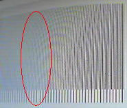 | Figure 4. Barrel distortion |
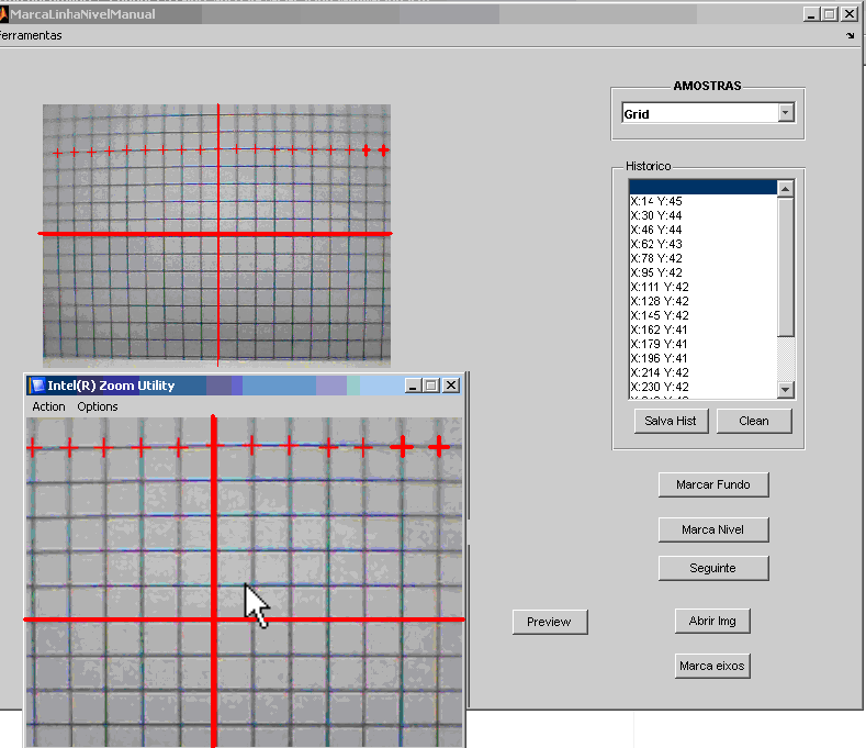 | Figure 5. Correcting distortions through a grid intersection |
For instance, in a  grid (Figure 6), for the twenty-five intersections (measured from the center of the grid, in pixels with distortion), an array
  of heights is generated. A member
  of
of  is the height calculated from the vertical line in the center of the image. In this example, as the actual distance from each line with respect to the others is
  , the heights are easily calculated:
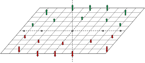
  . In the Figure 7 each square has
  pixels, an arrow may be null (small circles), positive (
 or
or  ) if pointing upwards, or negative otherwise. It represents the correspondence between the distorted coordinates of an intersection in pixels and the actual height, without deformation, in centimeters.
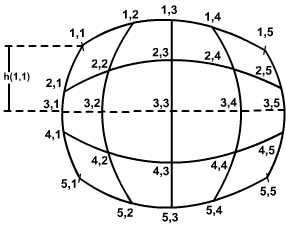 | Figure 6. A grid pixel/cm correcting a barrel distortion |
 | Figure 7. Distorted coordinates × actual height without deformation |
Although this relationship between the distorted coordinates and the non-distorted height is known, it is difficult to correct accurately all the points of the image. In fact, the intersection points are corrected, but it is necessary to approximate lines in order to correct the other points. This results in an exponential growing of intersections. The camera from DUVE captures  centimeters of the collecting device and therefore just 1mm between the lines implies 81600 points. Nevertheless, since the relationship distorted-coordinate/actual-height has a constant behavior, an interpolation based on Delaunay triangulation [13] is applied with third degree polynomials to obtain new points between the intersections. These new points are stored in an array
  , and as long as the distance between the camera and the collecting device remains unchanged, new interpolations are not required because all values are already in
  . A function
 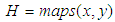 maps the original distorted points (in pixels) to the corresponding non-distorted heights (in centimeters).
  is graphically represented in the figures 8 and 9. A value from
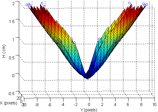
  is not the actual height of the product level due to the collecting device bottom height. The level is
 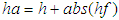 , where
  is the obtained level height, and
  is the bottom height (Figure 10).
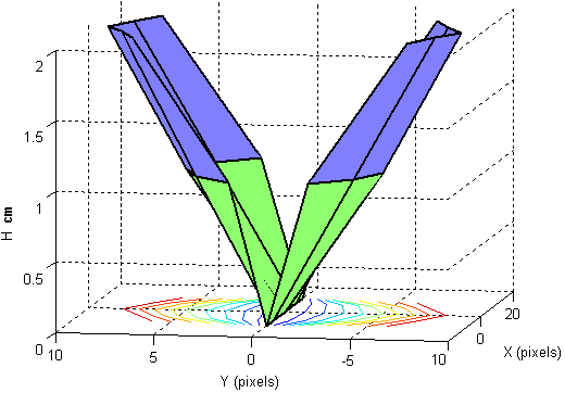 | Figure 8. H absolute value |
 | Figure 9. H and pixels/centimeters |
 | Figure 10. Interpolation process |
2.4. The LMM Identification of the Lateral Edges
The cornerstone of this process is the barcode identification. The top left and bottom right coordinates are used in the search of the horizontal lines that lie close to the projection of the barcode center point, the dotted line in Figure 11. The horizontal component of the Sobel filter (directly on the initial image) was solitarily used in order to verify the edges horizontal lines. Unfortunately, this resulted in bad defined edges with a lot of noise. In order to try to reduce these noises a median filter was applied, but this worsened the sharpness of the edges.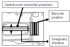 | Figure 11. Searching for a lateral edge |
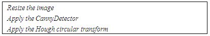
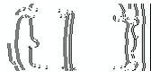
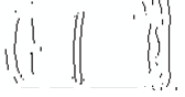
This problem was solved by the VILEMEM methodology employing a threshold  in the binary representation of a window of the image, and then applying the Canny detector which results in increased sharpness. As a Canny detector does not have specialized masks for detecting vertical or horizontal lines, the horizontal component of the Sobel filter and a median filter are applied to reduce noise. Eventually, a constant sized imaginary window passes through the image while the threshold is compared to the quantity of pixels (inside the window). This allows selecting the lateral edges among the possible candidates.With this combination of filters, the LMM identification of lateral edges process have shown robustness and efficacy in some experiments with DUVE, exhibiting promising results in extracting horizontal and vertical edges. Figures 12, 13, 14, 15, 16 and 17 show a sequence of application of these algorithms in an actual experiment using DUVE.
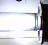 | Figure 12. Captured image |
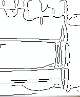 | Figure 13. Canny detector |
 | Figure 14. Sobel filter |
 | Figure 15. Median filter |
 | Figure 16. Window method |
 | Figure 17. Edges found |
Whenever the dimensions of the collecting device are known it is possible to apply a straightforward method to find the horizontal line (with the searched dimension), which is the closest to the horizontal projection of the barcode center point. Afterwards, a constant sized imaginary window is used (the window height is approximately equal to the lateral edges of the collecting device), which contains a particular pixel and some bordering pixels. This window may continually shift vertically through the image at a rate of one pixel per step. This is the VILEMEM ImaginaryWindow method. In experiments with DUVE this imaginary window was set as a rectangular area about half the height of the image, and all pixels in it were computed (sum of the horizontal projections of the window). If this sum is bigger than  then the area is considered as a possible edge or else the imaginary window is displaced up or down (depending on which edge is being searched) and the sum is again compared to
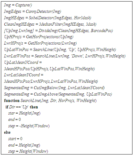
  .The LMM identification of the lateral edges process is based on the Algorithm 1. The experiments with DUVE have demonstrated that the use of the Sobel filter, the Canny detector and the ImaginaryWindow method together is an easy and very effective way to detect lines with known size and orientation. One of its main advantages is the detection of lines that are not perfectly straight.
Algorithm 1. Detection and segmentation of lateral edges
 |
| |
|
Some methods, such as the Hough transform for lines, basically detect “perfect'” straight lines. Another important advantage of this algorithm is its low cost. Its main disadvantage is that it requires knowing in advance the approximate dimension of the line being searched in order to correctly set  , and to delimitate the region of search. This disadvantage is less serious if the environment is controlled. Such as DUVE, the majority of the environments for real crude oil distillation processes are controlled.The Algorithm 1 calculates the straight lines
  , where
  is a constant and
  is the mean of the
  values that belong to the lateral edge. The SearchLine function selects the lateral edges among the possible candidates. The imaginary window is displaced by one pixel towards the top or the bottom. When the lines that represent the edges (calculated by the method of least squares) are found, the regions of the image above and below the detected edges are removed. This reduces the search space and obviously the cost of the algorithm.
2.5. The LMM Bottom Identification
The localization of the barcode reduces the search region of the bottom, whose main descriptor is an ellipse (a distortion from the circle of the bottom) captured by the camera. The Hough transform uses a voting procedure to find line [14], circle [15], ellipse [16], parabolic [17] etc. To detect a line, the idea is to identify linear or pseudolinear groups of disconnected points and intersected lines. A line 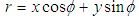 has
has  and
and  as the unknown parameters to be found. If this line intercepts a point
  then it can be solved with different values for
  and
and  . Thus, each point
  in the image can be associated with a set of values for
  and
and  . This set forms a sinusoidal curve in the space
  . As for each point in the image there is a related curve, the whole image has a large number of sinusoidal curves, which normally converge to a common point. Thus, a pair
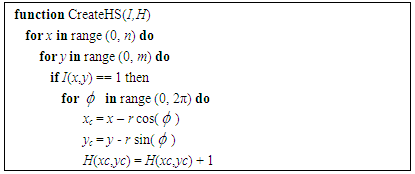
  from the sinusoidal convergence point indicates an inclination and a position r belonging to a line that can be drawn through the dots in the image.The Hough transform may be generalized to detect groups of points belonging to a curve, but this increases the complexity of the algorithm whether the defining function has too many independent variables (such as for ellipses). A modification of Hough transform for circles and ellipses detection has been well studied [18-21], as well as some methods reducing the complexity of the Hough transform for ellipses in unknown environments have been developed [22], [23]. In this context, VILEMEM proposes a simple and efficient method that transforms the original image to a circumference, reducing the computational effort. Indeed, since the axis of the bottom ellipse is parallel to the horizontal and vertical main axis of the captured image, then it is possible to resize the image and transform the ellipse in a circumference.The Algorithm 2 generates a Hough space, a two-dimensional array having the same size of the original image. The input I is a
  binarized image and the output
  is a
is a  array. The indexes from the columns and rows represent the possible values of the circumference center coordinates
  . All the cells
  , which represent centers of circumferences (with radius
  ), going through the point
  , are incremented in the Hough space. The cells with higher values point out the most probable centers of circumferences. The gradient method is used to search the higher values in the Hough space array.
Algorithm 2. Generating a Hough space
 |
| |
|
The abridged Algorithm 3 identifies the bottom of a collecting device. A bilinear interpolation helps the image resizing, and the m × n actual image is fitted in another 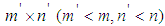 . The Canny detector removes the low frequency pixels from the image. The Hough transform for circles detects all pixels belonging to circumference candidates in the image. The Hough space is built (via Algorithm 2) and the obtained cells with higher values are the candidate centers for the circumferences. [23], for instance, focuses on an application of Hough transform for circumferences, whose centers and perimeters are detected after the Hough algorithm had been applied, and the highest value (point of maxima) of the Hough space array represents the best point to be a center of a circumference. In VILEMEM, the center of a corrupted circumference corresponds to the point of higher concentration of intersections in the Hough space. Thus, when the circumference center had been detected it is mapped back in the ellipse center via the application of the inverse process of resizing and the right vertical tangent of the circle will represent the bottom side of the collecting device.
Algorithm 3. Identifying the bottom of a collecting device
 |
| |
|
2.6. The LMM Detection of the Current Level
The identification of the bottom provides a hint to the visualization of the lateral edges, which are a benchmark to identify the measurable region. The level is a line in this region, which has three likely visualizations according to its localization with regard to the focal axis of the camera. The current height of the liquid is considered as the intersection between the lateral edges and the level-line. The level is assigned to a right and a left position of the intersections, and the final level is calculated as the mean of these two measures. The search region can be reduced through two cuts on the image after the bottom identification. As the level goes up while the liquid is dripping from the spout, the area below the last detected level might be theoretically discarded. Nevertheless, as the liquid may oscillates due to the impact of dripping, for safety sake a first cut in the image is done only at  pixels above the last detected level (
 is a predefined constant). A second cut is
  pixels wide,
  meaning the lower search limit for the next level detection (when the threshold
  is reached). Thus, the search region obtained by the discard of upper area (
 ) and lower area (
 ) can still be improved through the search of possible vertical intersections in the split left and right regions using the ImaginaryWindow method starting from the top of the restricted search region.
3. Measuring Fluid Levels through VILEMEM
During the development of VILEMEM, three algorithms were implemented and tested. Mishaps detected during some DUVE experiments have been solved in the VILEMEM enhanced algorithm. The first algorithm was based on the LMM identification of lateral edges, the second on the use of a set of frames and the third algorithm on the removing of irrelevant pixels.
3.1. An Algorithm Based on the Identification of Lateral Edges
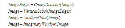
This algorithm uses Sobel filter and Canny detector through a vertical mask. The Canny detector is applied to detect the edges of the Image (Figures 18, 19) and the vertical component of the Sobel filter is applied to extract the vertical lines of the Image (Figure 20). A median filter is applied to reduce the noise of the Image (Figure 21). The ImaginaryWindow method is also used to detect and to segment the level-line, but improved to detect vertical lines.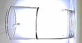 | Figure 18. Image |
 | Figure 19. Canny detector |
 | Figure 20. Sobel filter |
 | Figure 21. Median filter |
The main advantage of the Algorithm 4 is its swiftness due to its low computational cost and the straightforward insertion of the Canny detector, the Sobel filter and a median filter. The main disadvantages are due to the concomitant use of two processes for edge detection that increase the image noises (requiring a median filter to improve the final result). This means to accept a rough measurement of the level-line, which decreases the accuracy of the method. Thus, the error rate may be considerable and, in some frames, the level could not be measured. As only one frame is used to detect the level, in experiments with DUVE the levels from some images were not detected.Algorithm 4. Level measurement based on identifications of edges
 |
| |
|
3.2. An Algorithm Based on Sets of Frames
The Algorithm 5 uses a set of frames to detect the level-line, with six frames extracted from every thirty frames. In DUVE it implies 2 seconds of video with an approximated capture rate of 16 fps. This means that one frame is selected to calculate the level-line at every  second. The mean
  of the heights (of the level-lines detected in each of the six selected frames) is considered the actual level-line. If the level had not been successfully detected in a selected frame f, then f is discarded and not computed in
  .
.Algorithm 5. Using a set of frames
 |
| |
|
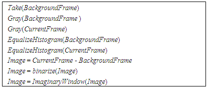
Histogram equalization is used to increase the contrast of the image, improving the level-line definition. Frame subtraction is calculated between a current frame and a background frame (the first is grabbed with the empty collecting device). This operation removes static elements of the image that interfere in the level detection. The function Gray (in second and third lines of the algorithm 5) converts a RGB image into a gray level image (Figures 22a and 22b). The function EqualizeHistogram does an equalization of the histogram of an image (Figures 22c and 22d). The sixth line of the algorithm subtracts the background frame from the current frame; the seventh line binarizes the result of this subtraction and the eighth line detects and segments the level line using the ImaginaryWindow method (Figure 22e).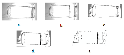 | Figure 22. Experiments using algorithm 5 |
3.3. An Algorithm Based on the Removal of Irrelevant Pixels
The Algorithm 6 removes irrelevant pixels (with high gray level, nearly white), and applies the subtraction method from a background frame. In this approach the pixels are removed according to the standard deviation  . It is considered that the most relevant Luminance Values Lv, found by the fifth line in algorithm 6, are below the limit Lv(1).
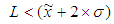 | (1) |
Algorithm 6. Removing irrelevant pixels
 |
| |
|
The pixels with values close to 0 are relevant for the level-line whereas the pixels near 255 are relevant for the background of the image. The Figure 23a shows an original image in grayscale and the Figure 23b shows the resulting image after applying the process removing non relevant pixels. If relevant pixels are selected by mistake as irrelevant and then removed, the level-line would be fragmented. The ClosingMorphologicalOperator was included to join these fragments. Thus, the Canny detector is used and eventually the level line is detected using the ImaginaryWindow method.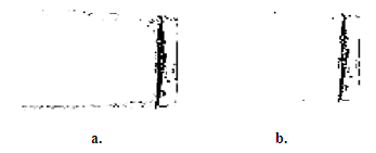 | Figure 23. Removing irrelevant pixels |
The function Gray in algorithm 6 converts a RGB image in a gray level image (Figures 24a and 24b). Figure 24c shows the result of the fourth line of algorithm 6. The pixels not accomplishing (1) become white (255) and the others black (0), and the final outcome is a binary image (Figure 24d). The ClosingMorphologicalOperator is a transformation that fills holes and blocks narrow values by applying a structuring element (with size similar to the holes and values). Applying this operator to an image A through a structuring element B (2) means initially applying a dilation in A and then an erosion, both using B. Figure 24e shows the image after this operation.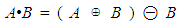 | (2) |
Removing noise is done by evaluating the 8-neighbors of each pixel. For instance, if a pixel has less than X black neighbors it is considered to be noise and removed (Figure 24f). Canny detector is applied to extract edges (Figure 24g) [24], [25]. The main advantage of this algorithm is its reliability and performance with regards to Algorithms 4 and 5. It uses several frames to calculate the height of the liquid level. In DUVE experiments, all frames had the level detected. The main disadvantage is its high computational cost due to the parallel running of several image-processing algorithms.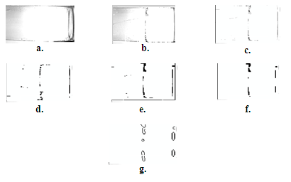 | Figure 24. Experiments using algorithm 6 |
3.4. The VILEMEM Algorithm
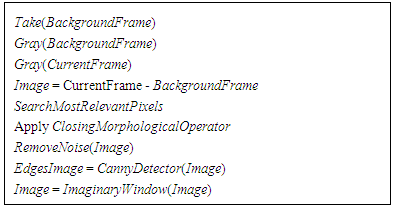
The Algorithm 7 improves the three precedent algorithms and solves their drawbacks. For instance, a tricky problem is when the liquid is (almost) transparent, causing a low image contrast of the level-lines. To solve this kind of problem, a particular method for enhancing image definition was developed. Assuming that the frame rate of a camera is high enough to get consecutive frames with a small level displacement, the merge of these frames would result into an “averaged image” with more accurate level-line. In the VILEMEM Algorithm the SumArray is sized as the restricted region of search (using p1 to discard the upper area and p2 to discard the lower area). TotalFrames is the total number of frames used for the average operation. In GetLastFrame the idea is to acquire the last frame captured by the grabber and add each element of the array to the element of SumArray (with the corresponding indexes). The normalization of SumArray is calculated as shown in (3).Algorithm 7. The VILEMEM Algorithm
 |
| |
|
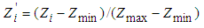 | (3) |
 is the
  element of SumArray,
  is its maximum element, and
  is its minimum element. The median filter reduces noises. SaturatePixels saturates the highest and the lowest pixels of the normalized sum array by an empirical value (for instance, 3% was obtained as an ideal value in DUVE), which improves the contrast. Categorizing the search region helps the identification of the left and the right intersections between the level-line and both the lateral edges. The image is categorized in three sections with the same size (Figure 25) and the central region (B) is discarded from the search. VertIntersections searches for the possible vertical intersection in the regions A and C using the ImaginaryWindow method, starting from the top of the restricted search region. CorrectDistortion corrects the distortion of the Image using the LMM correction of image distortions. Normalization is used instead of the mean calculation of
  . In fact, normalization has proven to be more helpful and accurate than the mean calculation. Indeed, during mean calculation some relevant pixels representing edges of the image may be discarded. This does not occur in the normalization approach.
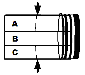 | Figure 25. Searchable area |
The Figure 26 emphasizes the efficiency of the normalization approach using three examples of grabbed frames. The two binarized results were obtained with both edge enhancing methods, with a threshold  to binarize each case. Our normalization approach generates a successful accurate representation of the actual edge with a suitable computational cost for a real-time edge enhancement. The VILEMEM Algorithm is fast and has a low computational cost too. One of its important advantages is the application of several frames to measure the level-line, which increases its reliability. In DUVE experiments the best results were obtained using this algorithm with all measurable variables (including
  and MAE). The main disadvantage of this algorithm is that it requires a high rate of capture of several frames in order to be applied in the normalization approach.
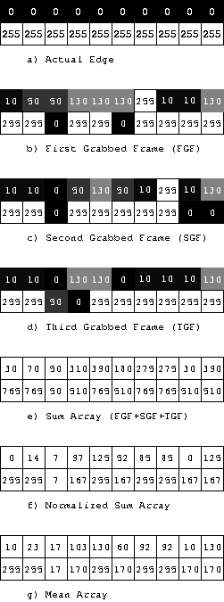 | Figure 26. Actual edge and samples |
4. Main Results
The VILEMEM methodology was tested through several DUVE experiments using crude oil samples. The algorithms presented in this paper were continuously enhanced until VILEMEM confirmed itself as an effective measuring methodology for crude oil distillation processes. In DUVE it was used three kinds of oil falling speeds: the slow falling  (drops), the medium falling
  (moderate stream) and the high falling
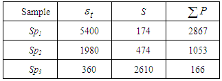
  (streaming). Table 1 illustrates an experiment using 86020, 31613 and 4981 frames for
  ,
,  and
and  , respectively. The elapsed time (in seconds) of the experiment is represented by
 ,
,  is the estimated falling speed of the liquid (in ml/second), and
  represents how many points were highlighted (to compare against the points of the level detected by our methodology).
Table 1. Slow, medium and high fallings
 |
| |
|
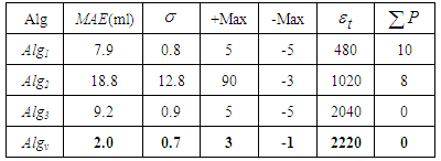
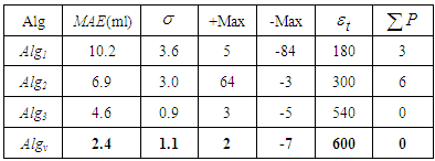
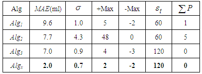
Tables 2, 3 and 4 show the mean absolute error MAE, the standard deviation (), the lower and upper max errors measured in mm (-Max and +Max), the elapsed time (
 ), and the quantity of points where the level was not detected (
 ), in relation with the error analysis. Alg1 is the algorithm based on lateral edge identification; Alg2 is the frame based algorithm; Alg3 is the removing pixels based algorithm; and Algv is the VILEMEM Algorithm.
Table 2. Error analysis for slow falling
 |
| |
|
Table 3. Error analysis for medium falling
 |
| |
|
Table 4. Error analysis for high falling
 |
| |
|
An error (MethodologyLevelValue - ActualLevelValue) is positive whenever the level detected is higher than the actual position, and it is negative otherwise. The mean of an error is calculated using the absolute value of the errors. +Max and -Max are in pixels. As shown by the tables 2, 3 and 4, the values of the MAE and  corroborate to emphasize the robustness and effectiveness of VILEMEM for crude oil level measurements. For instance, with a collecting device with radius of 3.3cm, the minimum detectable volume calculated was 3.4 ml, with the mean
  computed by VILEMEM at every evaluated point approximately equal to 1mm. With a collecting device with radius of 4.5cm, the minimum detectable volume was 6.3 ml. These results have completely corroborated to all our expectations.
5. Conclusions
The dynamic measurement of fluid level is a complex task. This complexity increases when the liquid being monitored is flammable or has changeable densities. The most widely known level measurement methodologies require periodic recalibrations of sensors and these recalibrations must be done by human interventions. This paper proposed a computer-based methodology for liquid level measurement. This new methodology, named VILEMEM, is a synchronous density-independent and non-contact approach that does not require periodical sensor recalibrations. VILEMEM incorporates algorithms, methods and processes designed for all level measurement activities. This paper also presented DUVE, a distillation unit built especially to test VILEMEM using experiments with crude oil samples. The results of these experiments have demonstrated that VILEMEM is safe, truthful and adequate to actual crude oil distillation activities. VILEMEM is based on the use of Hough transform, Canny detector and enhancements of image processing techniques.VILEMEM algorithms, methods and processes met all requirements of safety, speed, cost and robustness during the experiments. VILEMEM is non-intrusive (liquids are not touched), has a low application cost and may be used for other liquids besides crude oil. VILEMEM uses a normalization approach that is more accurate and faster than the usual calculating approach (widely applied in level measurement methodologies). The concomitant use of Canny detector, Sobel filter, median filters and the ImaginaryWindow method is the cornerstone of the low-cost and simplicity of the VILEMEM implementation in real level measurement processes.
References
| [1] | M. Jeffries, E. Lai and J. B. Hull. Fuzzy flow estimation for ultrasound-based liquid level measurement. Engineering Applications of Artificial Intelligence, vol. 15, 31-40, 2002. |
| [2] | S. Chakravarthy, R. Sharma and R. Kasturi. Noncontact level sensing technique using computer vision. IEEE Transactions on Instrumentation and Measurements, vol. 51 (2), 353-361, 2002. |
| [3] | C. Gaber, K. Chetehouna, H. Laurent, C. Rosenberger, and S. Baron. Optical sensor system using computer vision for the level measurement in oil tankers. In Proceedings of the ISIE, Cambridge, UK, 1120 – 1124, July 2009. |
| [4] | P. Hough. Machine analysis of bubble chamber pictures. In Proceedings of the International Conference on High Energy Accelerators and Instrumentation, Geneva, Switzerland, 554-556, September 1959. |
| [5] | M. Fokkinga. The Hough transform. Journal of Functional Programming, vol.21 (2), pp.129-133, 2011. |
| [6] | J. Canny. A computational approach to edge detection. IEEE Transactions on Pattern Analysis and Machine Intelligence, vol 8, pp 679-698, 1986. |
| [7] | W. Mcilhagga. The Canny Edge Detector Revisited. International Journal Of Computer Vision, vol.91 (3), pp.251-261, 2011. |
| [8] | S. Imrith, M. Heenaye. International Journal of Image Processing, vol 5 (3), pp 321-335, 2011. |
| [9] | H. B. C. Bins. Manufacturing Processes: Oil Refining, Occup Med. Oxford Journal, vol. 29, 113–116, 1979. |
| [10] | G. N. Abaev. A Computer Suite for Simulating Oil Product Fractional Distillation. Chemical and Petroleum Engineering, vol. 35 (4), 202–205, 1999. |
| [11] | H. Al-Muslim. Thermodynamic Analysis of Crude Oil Distillation Systems. International Journal of Energy Research, vol. 29, 637–655, 2005. |
| [12] | C. Pei-Yin, H. Chien-Chuan, S. Yeu-Horng, C. Yao-Tung. A VLSI Implementation of Barrel Distortion Correction for Wide-Angle Camera Images. IEEE Transactions on Circuits and Systems II: Express Briefs, vol. 56(1), pp.51-55, 2009. |
| [13] | B. Delaunay. Sur la sphére vide. Izvestia Akademii Nauk, vol. 7, 793–800, 1934. |
| [14] | R. C. Gonzalez and R. E. Woods. Digital Image Processing, second ed., McGraw Hill, 2002. |
| [15] | B. Batchelor and P. F. Whelan. Intelligent vision systems for industry, Springer, New York, USA, 2002. |
| [16] | X. Yonghong and J. Qiang. A New Efficient Ellipse Detection Method. Proceedings of the 16th International Conference on Pattern Recognition, IEEE: Quebec, Canada, 957–960, 2002. |
| [17] | D. Gonzalez-Ortega, M. Martinez-Zarzuela, F. J. Diaz-Pernas; J. F. Diez-Higuera, M. Anton-Rodriguez, D. Boto-Giralda, J. M. Hernandez-Conde. Real-time system for elliptical based face detection. Pattern Recognition and Image Analysis, vol. 19 (4), 647–655, 2009. |
| [18] | L. Jiang. Efficient randomized Hough transform for circle detection using novel probability sampling and feature points. Optik - International Journal for Light and Electron Optics, vol. 123 (20), 1834 – 1840, 2012. |
| [19] | W. Lu, J. Yu, J. Tan. Direct Inverse Randomized Hough Transform for Incomplete Ellipse Detection in Noisy Images, Journal of Pattern Recognition Research, vol. 9 (1), doi:10.13176/11.512 , 2014. |
| [20] | R. K. K. Yip, P. K. S. Tam, D. N. K. Leung. Modification of Hough transform for circles and ellipses detection using a 2-dimensional array, Pattern Recognition, vol. 25 (9), 1007 – 1022, 1992 |
| [21] | P. K. Ser, W. C. Siu. Novel 2-D Hough planes for the detection of ellipses. Proceedings of the IEEE International Symposium on Speech, Image Processing and Neural Networks, IEEE: Hong Kong, China, 527–530, 1994. |
| [22] | S. M. Aguado, E. Montiel and M. S. Nixon. Ellipse detection via gradient direction in the Hough transform. Fifth International Conference on Image Processing and its Applications, Edinburgh, UK, 375–378, 1995. |
| [23] | T. Peng. Detect circles with various radii in grayscale image via Hough transform. http://www.mathworks.com/matlabcentral/fileexchange/9168. Accessed: 1st May, 2015. |
| [24] | R. Biswas, J. Sil. An Improved Canny Edge Detection Algorithm Based on Type-2 Fuzzy Sets. Procedia Technology, vol. 4, 820 – 824, 2012. |
| [25] | B. Bansal, J. Saini, V. Bansal, G. Kaur. Comparison of various edge detection techniques. Journal of Information and Operations Management, vol. 3(1), 103-106, 2012. |
 Abstract
 Reference
 Full-Text PDF
 Full-text HTML