Douzi Youssef 1, Benabdellah Mohammed 1, Azizi Abdelmalek 1, Hajji Tarik 2, Jaara El Miloud 2
1Laboratoire d’Arithmétique Calcul Scientifique et Applications, Université Mohammed Premier, Maroc
2Laboratoire de recherche en informatiques (LaRI), Faculté des Sciences d’Oujda (FSO), Université Mohammed Premier (UMP), Oujda, Maroc (LaRI/FSO/UMP)
Correspondence to: Hajji Tarik , Laboratoire de recherche en informatiques (LaRI), Faculté des Sciences d’Oujda (FSO), Université Mohammed Premier (UMP), Oujda, Maroc (LaRI/FSO/UMP).
| Email: |  |
Copyright © 2015 Scientific & Academic Publishing. All Rights Reserved.
Abstract
We will show in this work, the use of artificial neural networks (ANN) as a new way of doing zoom operations on digital images. The objective is to make the presentation and description of four new approaches to zoom based on the use of ANN. These approaches will allow us to achieve regional and global zoom on a digital image. We will use a supervised learning algorithm for our ANN. We will use a database of learning formed by a set of digital images and their versions zoomed carefully by software zoom. We will also even a brief on ANN, their working principle and the famous zoom digital images methods. In this work, we will also prove the effectiveness of ANN as a good solution to the problem of restoring digital images defective due to zooming.
Keywords:
Component, Zoom, ANN, Ddigital Images, Restoring, Learning
Cite this paper: Douzi Youssef , Benabdellah Mohammed , Azizi Abdelmalek , Hajji Tarik , Jaara El Miloud , Zoom and Restoring of Digital Images with Artificial Neural Networks, Computer Science and Engineering, Vol. 5 No. 1, 2015, pp. 14-24. doi: 10.5923/j.computer.20150501.03.
1. Introduction
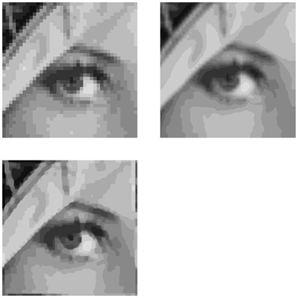
The zoom is a standard operation that can be performed on a digital image, its goal is to appear in the clear objects in an image have difficulties viewing. To solve this problem, we try to find ways to expand the regions, or fully images without loss of information at the end to recognize the objects in the image, or to make treatments on these objects. You can define the order of zoom as a variable to measure the degree of zooming, other words, the ratio between the size of zoom and the size of the original image.We will begin this work, by this introductory section, which is describe zooming and their importance in the field of digital image processing, the types of zoom that can be applied in a digital image, state of the art to expose the famous zoom images methods, a brief introduction on the functioning of ANN and at the end of this section we will outline the main features of our approach. Finally, we will describe in the methodology section, the approach used and the different algorithms and results.A. Partial ZoomlWe denote by the partial zooming, a zooming operation that can be performed on a block or a region of a digital image. The following figure shows an example of partial zoom of order X4: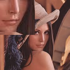 | Figure 1. Partial Zoom |
B. Global ZoomWe denote by the global zoom, zooming applied entirely on a digital image. The following example shows an operation global zoom 4X Sequence: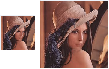 | Figure 2. Global Zoom |
C. Artificial Neural NetworkThe neural network is inspired by biological neural system. It is composed of several interconnected elements to solve a collection of varied problems. The brain is composed of billions of neurons and trillions of connections between them. The nerve impulse travels through the dendrites and axons, and then treated in the neurons through synapses. This results in the field of ANN in several interconnected elements or belonging to one of the three marks neurons, input, output or hidden. Neurons belonging to layer n are considered an automatic threshold. In addition, to be activated, it must receive a signal above this threshold, the output of the neuron after taking into account the weight parameters, supplying all the elements belonging to the layer n +1. As biological neural system, neural networks have the ability to learn, which makes them useful. The ANN are units of troubleshooting, capable of handling fuzzy information in parallel and come out with one or more results representing the postulated solution. The basic unit of a neural network is a non-linear combinational function called artificial neurons. An artificial neuron represents a computer simulation of a biological neuron human brain. Each artificial neuron is characterized by an information vector which is present at the input of the neuron and a non-linear mathematical operator capable of calculating an output on this vector. The following figure shows an artificiel neural [1]: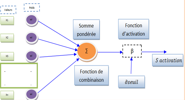 | Figur 3. Artificial neuron |
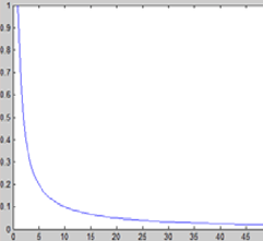
The synapses are Wij (weights) of the J neurons; they are real numbers between 0 and 1. The function is a summation of combinations between active synapses associated with the same neuron. The activation function is a non-linear operator to return a true value or rounded in the range [0 1]. In our case we use the sigmoid function [1]: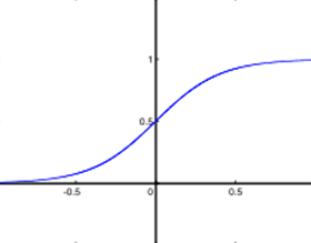 | Figure 4. Sigmoid function |
An artificial neural network is composed by a collection of artificial neurons interconnected among them to form a neuronal system able to learn and to understand the mechanisms. Each artificial neural network is characterized by its specific architecture; this architecture is denoted by the number of neurons of the input layer, the number of hidden layers, the number of neurons in each hidden layer and the neurons number in the output layer. A layer of neurons in a neural network is a group of artificial neurons, with the same level of importance, as is shown in the following figure [1]: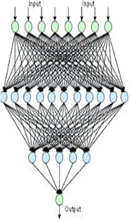 | Figure 5. Artificial neural network |
The operating principle of ANN is similar to the human brain; first, it must necessarily pass on the learning phase to record knowledge in the memory of the artificial neural network. The storage of knowledge is the principle of reputation and compensation to a collection of data that forms the basis of learning. We have several algorithms that can teach an artificial neural network as backpropagation.The backpropagation is a method of calculating the weight for network supervised learning is to minimize the squared error output. It involves correcting errors according to the importance of the elements involved in fact the realization of these errors: the synaptic weights that help to generate a significant error will be changed more significantly than the weights that led to a marginal error. In the neural network, weights are, first, initialized with random values. It then considers a set of data that will be used for learning.D. Methods of zoom digital imagesThere is a wide range of approaches invented in the intention to treat the subject of zoom digital images. F. Guichard and F. Malgouyres introducing an interpolation method based on a calculation of the total variation of the image. The method of the paper is similar to those of conventional restoration where you can enjoy an a priori knowledge on the image to obtain (eg belonging to BV). Hence the idea to formulate the problem of estimating the image w from u controlling the regularity of w:  is a term attachment or loyalty to the image data u - and
  is a regularization term, eg total variation. If
  is small, we will have a good fidelity data. If
  is increases, then will be a much more regular picture. In the case before us, the term fidelity can be expressed by the condition 1, which is belonging to the space
  It remains to choose a regularity measure for the term
 | Figure 6. Interpolation based on a calculation of the total variation of the image |
The results provided by the zoom by minimizing the total variation are rather satisfactory, they make a very acceptable visual quality, but we believe that some improvements have been possible in a few constraints renouncing Article membership  it was perhaps too strong an attachment to the data to remove the Gibbs oscillations. More generally, the interest of effective methods of interpolation is emphasized to increase the image resolution. There are many applications: printing with good image quality, increased resolution digital image acquisition devices (scanner, webcam, etc.). Conventional techniques based on the convolution of the image with a single core, bilinear or bicubic interpolation types have obvious limitations. However, define the problem of increasing resolution as an ill-conditioned inverse problem seems very interesting.
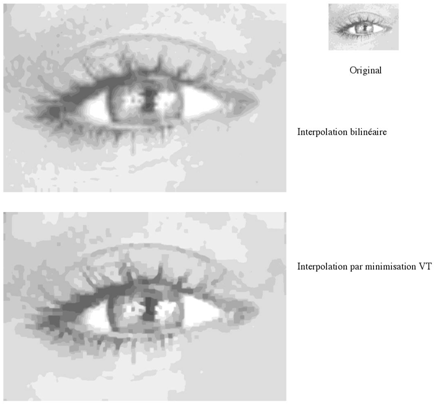 | Figure 7. Interpolation based on the convolution of the image |
E. Proposed methodIn this work, we will propose four approaches of exploitation of ANN to perform the zoom operations on digital images: • Recursive approach: using recursively an artificial neural network able to do the zoom of a digital image.• Serially approach: using a multilayer artificial neural network capable of generating a sequence of digital images representing a zooms for original image. • Parallel approach: Consist of instantiate a set of ANN share the input layer and the first hidden layer, and also share the learning process. • Hybrid approach: using the recursive approach to a neural network not fully connected.
2. Methodology
The principle of this method is to construct a neural network decompression, able to learn the zoom mechanism on digital images with the backpropagation algorithm. A. Recursive approach1) Principle of the approac In this approach multilayer ANN are used, with a larger than the input layer to output layer. The objective is to generate for each input block another block greater output, which represents a zoom for the input block. The following figure shows an artificial neural network characterized by the following structure:• An input layer, composed by two artificial neural capable of processing a digital image of a block formed of two pixels.• A hidden layer, formed by three artificial neurons. • An output layer, composed by four artificial neurons.The artificial neural network is capable of a zoom operation on a digital image to make the generation of the output a two times greater than image or block presented to the input of the neural networks. We denote by the architecture of a neural network, the number of neurons in the input layer, the number of hidden layers, the number of artificial neurons in each hidden layer and the number of neurons in the output layer.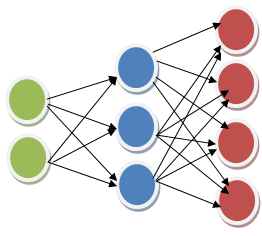 | Figure 8. ANN for the recursive approach |
One can write for example (2, 3, 4) to indicate the architecture of an ANN characterized by an input layer of two artificial neural, one hidden layer with a three artificial neural and output layer with four artificial neural. The artificial neural network (2, 3, 4) capable of operation in 2X zoom level one pass ; if we want to achieve a relatively high degree of zoom, then you should repeat the zoom operation on heavy generated block of the first propagation. For example, to make a 4X zoom operation level, then we must reiterate zooming twice: 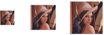 | Figure 9. Zooming with the recursive approach |
It is mainly used in this study two multilayer artificial neural network (2, 3, 4) and (2, 4, 16). The learning data base for this approach is comprised by a series of digital images and their zoomed versions. Zoomed versions of these images are constructed by MATLAB. The principle of the learning algorithm is highly unexpected of backpropagation, available for each image the zoomed version. And the image is subdivided into a suitable collection at the inlet of artificial neural network, in parallel; this operation must be repeated on the zoomed versions. Then calculated for each block its image by the artificial neural network and comparing the resulting output a with zooming and finally calculates the individual errors in each neuron block to update knowledge in the synapses of the artificial neural network.2) Learning AlgorithmThe learning algorithm of this approach is as follows: • Step 0: on subdivise chaque image I de la base d’apprentissage en blocs  de taille dépendante de la taille de la couche d’entrée du réseau de neurones artificiels. • Step 1: Initialize the connection weights (weights are taken randomly).• Step 2: Propagation entries entered the
  are presented to the input layer:
 | (1) |
• The spread to the hidden layer is made using the following formula: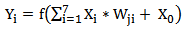 | (2) |
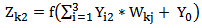
• Then from the hidden layer to the output layer, we adopt: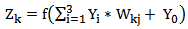 | (3) |
 And
And  are scalar;
 Is the activation function:
  | (4) |
• Step 3: Back propagation of errorat the output layer, the error between the desired output  and
and  output is calculated by:
 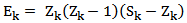 | (5) |
The error calculation is propagated on the hidden layer using the following formula: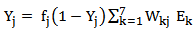 | (6) |
• Step 4: Fixed connection weights the connection weights between the input layer and hidden layer is corrected by: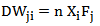 | (7) |
And | (8) |
Then, we change the connections between the input layer and the output layer by: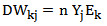 | (9) |
N is a parameter to be determined empirically.• Step 5 loops: Loop to step 2 until a stop to define criterion (error threshold, the number of iterations.The following figure shows the graph of convergence of the algorithm:3) Zoom algorithmThe zoom algorithm is as following• Step 1: subdividing the original image I into blocks  of size dependent on the size of the input layer of the neural network. • Step 2: we propagate each block
  in the artificial neural network:ο From the hidden layer to the input layer:
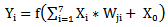 | (10) |
 | Figure 10. ANN (2 ; 3 ; 4) graph convergence |
ο From the hidden layer to the output layer 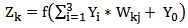 | (11) |
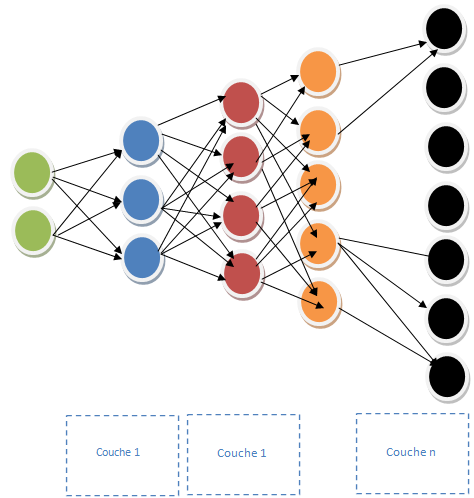
• Step 3: it is the reconstitution of the zoom from the blocks  generated by the artificial neural network.• Step 4: while the range of zoom applied is not yet complete then loupe to Step 1 with the zoom as an original image.B. Approach seriated1) Principle of the approach The principle of this approach is to build a multilayer artificial neural network, each layer represents a zoom operation for the input vector, the following figure explains this principle; it has a multilayer artificial neural network (2, 3, 4, and 5... n): The learning algorithm on this approach is relatively complicated. The principle of the learning algorithm is based on two axes: The basis of training data and back propagation algorithm. We will use the artificial neural network architecture (2; 3; 4; 16); the first hidden layer consists of three artificial neural it will not be used to capture a zoom; it will be used just for the more flexible artificial neural network. The second hidden layer composed by four artificial neurons will be used to capture a sequence 2X zoom. The third hidden layer artificial neural 16 will be used to capture a 4X zoom order for the block input. For each block of training data based zoom order there are n-1 respectively 2X, 4X. Each zoom will be used in the layer corresponding to the order size zoom. The following figure shows how to iterate
  on a single block
  which is present at the input of the artificial neural network, with
  zoom order 2X and
  zoom order 4X for the bloc
 | Figure 11. ANN for approach serially |
 | Figure 12. Learning algorithm |
2) Learning algorithm The following chart explains the principle of the algorithm: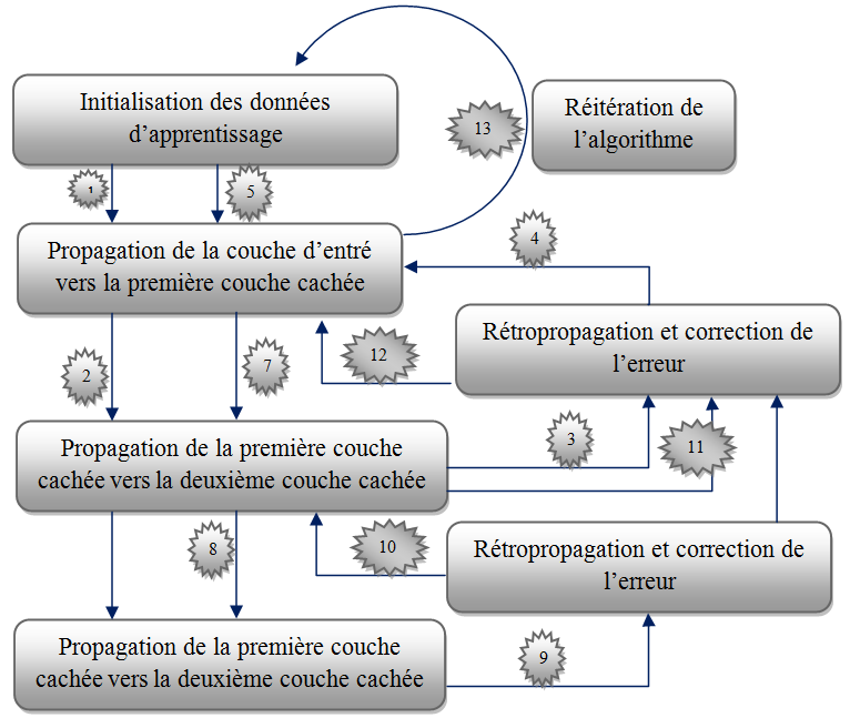 | Figure 13. Principle of the algorithm |
The algorithm is as following:• Step 0: subdividing the original image I into blocks  of size dependent on the size of the input layer of the neural network. • Step 1: Initialize the connection weights (weights are taken randomly).• Step 2: Propagation the entered
  presented to the input layer:
  | (12) |
The spread to the hidden layer is made using the following formula: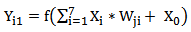 | (13) |
Then from the hidden layer to the output layer, we adopt: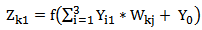 | (14) |
 And
And  are scalar;
  Is the activation function:
 | (4) |
• Step 3: Back propagation of error at the output layer, the error between the desired output  and
and  output is calculated by:
 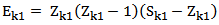 | (15) |
The error calculation is propagated on the hidden layer using the following formula: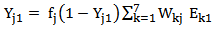 | (16) |
• Step 4: Fixed connection weights the connection weights between the input layer and hidden layer is corrected by: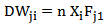 | (17) |
And | (18) |
Then, we change the connections between the input layer and the output layer by: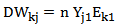 | (19) |
• Step 5: Propagation entries entered the  are presented to the input layer:
  | (12) |
The spread to the hidden layer is made using the following formula: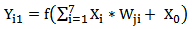 | (13) |
Then from the hidden layer to the next hidden layer, we adopt: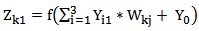 | (14) |
Then, propagation of the signal to the last hidden layer (output layer) by: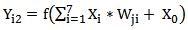 | (20) |
 | (21) |
• Step 6: Back propagation of errorat the output layer, the error between the desired output  and
and  output is calculated by:
 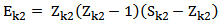 | (22) |
The error calculation is propagated on the hidden layer using the following formula: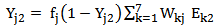 | (23) |
• Step 7: Fixed connection weights the connection weights between the input layer and hidden layer is corrected by: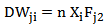 | (24) |
And | (25) |
Then, we change the connections between the input layer and the output layer by: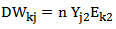 | (26) |
• Step 9: Back propagation of error at the output layer, the error between the desired output  and
and  output is calculated by:
 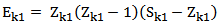 | (15) |
The error calculation is propagated on the hidden layer using the following formula: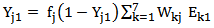 | (16) |
• Step 10: Fixed connection weights the connection weights between the input layer and hidden layer is corrected by: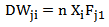 | (17) |
And | (18) |
Then, we change the connections between the input layer and the output layer by: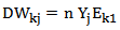 | (19) |
• Step 11 loops: Loop to step 2 until a stop to define criterion (error threshold, the number of iterations.The following figure shows the graph of convergence of the algorithm: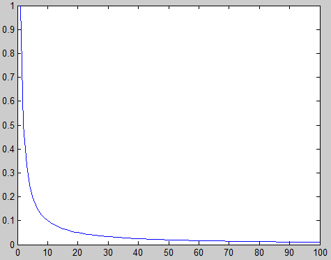 | Figure 14. Graph of convergence of the algorithm |
3) Zoom algorithm• Step 1: subdividing the original image I into blocks  of size dependent on the size of the input layer of the neural network. • Step 2: we propagate each block
  in the artificial neural network:ο From the hidden layer to the input layer first:
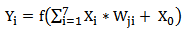 | (20) |
ο From the first hidden layer to cover the second layer: 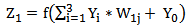 | (21) |
ο From the second hidden layer to the output layer: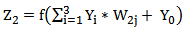 | (22) |
• Step 3: it is the reconstitution of the zoom from the blocks  generated by the artificial neural network in each hidden layer of the network.The following figure shows an example of a zoom of 4X and 16X order with an artificial neural network (2, 3, 4, 16): There is a loss of information due to regular saturation problem of neurons in the network. We can easily solve this problem by a simple filter or by the use of neural networks for restoring digital images.
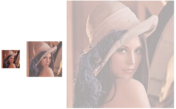 | Figure 15. Zooming with the serial approach |
C. Parallel approach 1) Principle of the methodThe objective of this zoom system is to construct ANN with a common root. This root is composed of the input layer and the first hidden layer. Each neural network has its own output layer corresponding size to order the zoom applied. The following figure shows two ANN (2, 3, 4) and (2, 3, 16) with part (2, 3) shared between them: 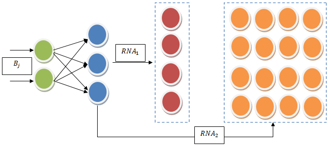 | Figure 16. ANN for approach parallel approach |
Learning is done by backpropagation parallel gardian on all ANN used. The idea is to get a first input block in the first artificial neural network and not move to the next block to get the block in wholes other ANN compose the zoom system.2) Learning Algorithm The following diagram shows the principle of the learning algorithm: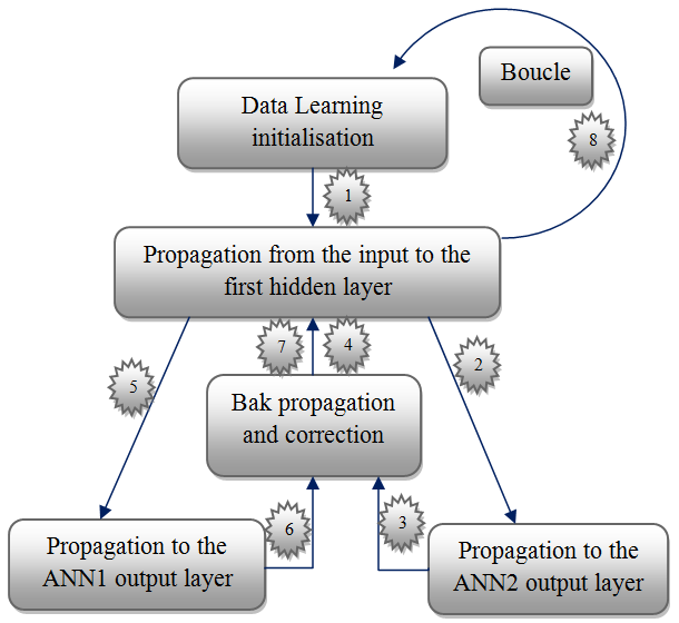 | Figure 17. Principle of the algorithm |
The algorithm is as follows:• Step 0: subdividing the original image I into blocks  of size dependent on the size of the input layer of the neural network. • Step 1: Initialize the connection weights (weights are taken randomly).• Step 2: Propagation entries entered the
  are presented to the input layer:
 | (23) |
The spread to the hidden layer is made using the following formula: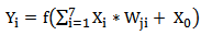 | (24) |
Then from the hidden layer to the output layer, we adopt: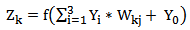 | (25) |
 And
And  are scalar;
 is the activation function:
 | (26) |
• Step 3: Back propagation of error at the output layer, the error between the desired output  and
and  output is calculated by:
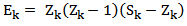 | (27) |
The error calculation is propagated on the hidden layer using the following formula: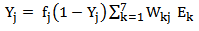 | (28) |
• Step 4: Fixed connection weights the connection weights between the input layer and hidden layer is corrected by: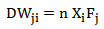 | (29) |
And | (30) |
Then, we change the connections between the input layer and the output layer by: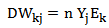 | (31) |
N is a parameter to be determined empirically.• Step 5 loops: Loop to step 2 until a stop to define criterion (error threshold, the number of iteration)The following figure shows the graph of convergence of the algorithm: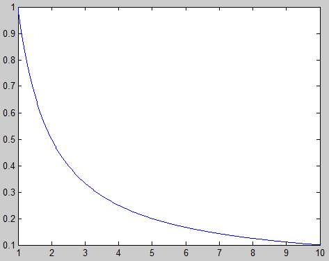 | Figure 18. Graph convergence ANN (2, 3, 4, 16) |
3) Zoom algorithm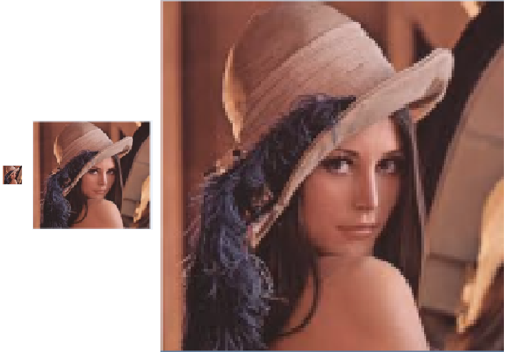 | Figure 19. Zooming with a parallel approach |
In this approach, we have orders to zoom is proportional to the input of the artificial neural network. In other words, the artificial neural network to be used is selected at the time of definition of the order of zoom. After the recognition of the order of zoom can be applied immediately make a simple propagation in the corresponding artificial neural network in this order zoom. The following figure shows an example of using this approach:D. Hybrid Approach1) Principle of the approachThe principle of this approach is exactly the same as the recursive approach. However, the difference is in the structure of artificial neural network used. Difference is reflected in the connections between neurons that are trying to generate some sort of normalization of the amount of knowledge stored in the network of artificial neuron. The objective of this approach is to increase the order of a digital image zooming, to solve the problem when trying to apply a zoom operation with a relatively large range of zoom, in this case, the image to lose much of its quality. The following figure shows an instance of this problem: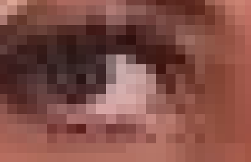 | Figure 20. Damaged blob |
The following figure shows the architecture of artificial neural network used in this work, Figure also shows the various connections between neurons used: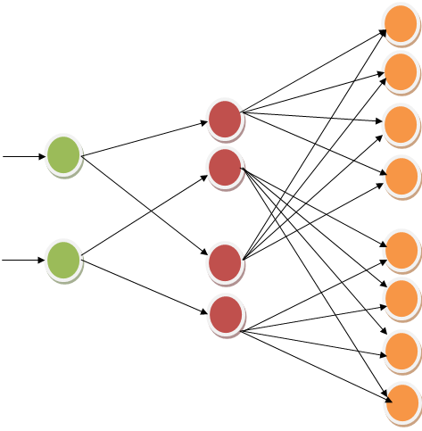 | Figure 21. ANN hybrid approach |
2) Learning Algorithm The learning algorithm associated with this method is similar to the glow of the recursive method except that this method will disable any connections between neurons in different layers of the artificial neural network. The following figure shows the graph of convergence of the algorithm: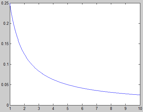 | Figure 22. Graph convergence for the hybrid approach |
3) Zoom algorithmWe did the same for the algorithm zoom than the recursive method; the original image is subdivided in a collection of blocks, and calculating for each order zoom postulated: 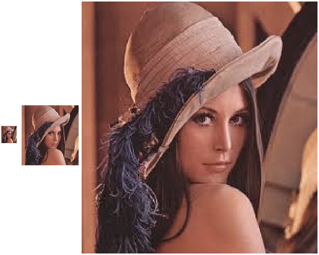 | Figure 23. Zoom with the hybrid approach |
3. Results
Are grouped in the following table the results for all the methods described previously. For each approach is the convergence rate mention by setting the number of iteration 1 billion. And also mention the zoom ratio recorded for each approach after 1000000000 iteration of the learning algorithm for sequence zoom 1024X. The zoom ratio is the percentage of similarity between the test image and the zoom picture generated by the artificial neural network. It should be noted that a range of zoom size <1024 all four methods generate pleasing results in terms of zoom ratio: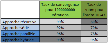 | Figure 24. Comparative results |
4. Conclusions
This study clearly shows the power of using ANN in several ways as an efficient approach capable of zoom operations on digital images. The structure, the learning algorithm, the learning base, the rate of convergence and order of zoom applied are all essential factors influence the effectiveness of using ANN to digital images zooming. The hybrid approach is very fast input to other approaches in terms of convergence time and at achieving zooming, and the more it is capable of generating zooms with monk swished.
References
| [1] | H. Tarik, J. El Miloud, “Digital Watermarking and Signing by Artificial Neural Networks”, American Journal of Intelligent Systems, Vol4, Num2, March 2014. |
| [2] | J. Clerk Maxwell, A Treatise on Electricity and Magnetism, 3rd ed., vol. 2. Oxford: Clarendon, 1892, pp.68–73. |
| [3] | I. S. Jacobs and C. P. Bean, “Fine particles, thin films and exchange anisotropy,” in Magnetism, vol. III, G. T. Rado and H. Suhl, Eds. New York: Academic, 1963, pp. 271–350. |
| [4] | K. Elissa, “Title of paper if known,” unpublished. |
| [5] | R. Nicole, “Title of paper with only first word capitalized,” J. Name Stand. Abbrev., in press. |
| [6] | Y. Yorozu, M. Hirano, K. Oka, and Y. Tagawa, “Electron spectroscopy studies on magneto-optical media and plastic substrate interface,” IEEE Transl. J. Magn. Japan, vol. 2, pp. 740–741, August 1987 [Digests 9th Annual Conf. Magnetics Japan, p. 301, 1982]. |
| [7] | M. Young, The Technical Writer's Handbook. Mill Valley, CA: University Science, 1989. |
| [8] | J. Fridrich. Methods for detecting changes in digital images. Proceedings IEEE Int. Conf. on Image Processing (ICIP’98), Chicago, USA, Oct. 1998. |
| [9] | Kodak. Understanding and Intergrating KODAK Picture Authentication Cameras.http://www.kodak.com/US/en/digital/software/imageAuthentication/. |
| [10] | D. Kundur and D. Hatzinakos. Towards a Telltale Watermarking Technique for Tamper-Proofing. IEEE International Conf. on Image Processing (ICIP’98) , Chicago, USA, Oct. 1998. |
| [11] | C.-Y. Lin and S.-F. Chang. A Watermark-Based Robust Image Authentication Using Wavelets. ADVENT Project Report, Columbia University, Apr. 1998. |
| [12] | J. Fridrich, M. Goljan & N. Memon. Further Attacks on Yeung-Minzer Fragile Watermarking Scheme. SPIE International Conf. on Security and Watermarking of Multimedia Contents II , vol. 3971, No13, San Jose, USA, Jan. 2000. |
| [13] | Julien Chable. Emmanuel Robles Programmation Android, de la conception au déploiement avec le SDK Google Android, New York, France, 2009. |
| [14] | F. Guichard et F. Malgouyres, Total Variation Based Interpolation, 2000-2001. |
 Abstract
 Reference
 Full-Text PDF
 Full-text HTML