G. A. Shidali, S. B. Junaidu, S. E. Abdullahi
Department of Mathematics, Ahmadu Bello University, Zaria, Nigeria
Correspondence to: G. A. Shidali, Department of Mathematics, Ahmadu Bello University, Zaria, Nigeria.
| Email: |  |
Copyright © 2015 Scientific & Academic Publishing. All Rights Reserved.
Abstract
Highest Response Ratio Next (HRRN) scheduling is a non-preemptive discipline, in which the priority of each job is dependent on its estimated run time and the amount of time it has spent waiting. Jobs gain higher priority the longer they wait, which prevents indefinite postponement (process starvation). Also, the jobs that have spent a long time waiting compete against those estimated to have short run times. HRRN prevents indefinite postponements but is neither preemptive nor suitable for priority systems. In this research, HRRN has been modified to accommodate external priority and to include preemption. Hence, a preemptive modified HRRN (PMHRRN) algorithm has been developed.
Keywords:
Starvation, Priority, Preemption, CPU scheduling
Cite this paper: G. A. Shidali, S. B. Junaidu, S. E. Abdullahi, A New Hybrid Process Scheduling Algorithm (Pre-Emptive Modified Highest Response Ratio Next), Computer Science and Engineering, Vol. 5 No. 1, 2015, pp. 1-7. doi: 10.5923/j.computer.20150501.01.
1. Introduction
Process scheduling is a fundamental function of an operating system [1]. The main concept is to share computer resources among a number of processes. Almost each computer resource is scheduled before use [2]. The Central Processing Unit (CPU) is one of the primary computer resources, so its scheduling is essential to an operating system’s design. Process scheduling is important because it plays an important role in effective resource utilization and the overall performance of the system. The aim of process scheduling is to assign processes to be executed by the processor over time, in such a way that meets system objectives such as response time, throughput and processor efficiency [3]. Scheduling algorithms can be classified by;1. Decision mode i.e. when do we take a scheduling decision? Categories of decision mode are non-preemptive and preemptive. 2. Selection function i.e. which process gets dispatched?Many criteria have been suggested for comparing CPU scheduling algorithms. Which characteristics are used for comparison can make a substantial difference in which algorithm is judged to be best. The following are some of the criteria.
1.1. CPU Utilization
This is the percentage of time that the processor is busy [3].The CPU should be as busy as possible [1].
1.2. Throughput
This is the number of processes that are completed per unit time [4]. The number of jobs processed per unit time should be maximized [5].
1.3. Turnaround Time
This is the interval between the time of submission of a process and the time of completion of that process [3]. The turnaround time should be minimized.
1.4. Waiting Time
This is the sum of the periods a process spends waiting in the ready queue [1]. Usually, the goal is to minimize the waiting time [4].
1.5. Response Time
This is the time it takes for a process to start responding [1]. It is the amount of time between the submission of a request and the first response to the request [4]. The response time should be minimized and users maximized in an interactive system [3].In this research, a framework to evaluate the effect of preemption on the performance of a hybrid scheduling algorithm Modified Highest Response Ratio Next (MHRRN) is proposed with the aim of minimizing waiting time, turnaround time and response time of processes.
2. Related Work
2.1. First-Come-First-Served (FCFS)
FCFS is the simplest scheduling policy. With this policy, when a process becomes ready, it joins the ready queue and when the currently running process completes, the process at the head of the ready queue, which has waited there for the longest time, is selected for execution [6].
2.2. Round Robin (RR)
A straightforward way to reduce the suffering of short processes is to use a time-sharing scheme, called Round Robin. The operating system assigns short time slices to each process and if the time slice allocated for a process is not enough for it to run to completion, the process is placed at the back of the ready queue while another process from the ready queue is dispatched.
2.3. Shortest Process Next (SPN)
The process with the shortest expected execution time is selected to run next.
2.4. Shortest Remaining Time (SRT)
The SRT policy is a preemptive version of SPN. In this case, the scheduler always chooses the process that has the shortest expected remaining processing time. When a new process joins the ready queue, RQ, it may in fact have a shorter remaining time than the currently running process. Accordingly, the scheduler may pre-empt the currently running process when a new process becomes ready [3].
2.5. Priority Scheduling
Each process is assigned a priority, and the process with the highest priority is allowed to run first [7]. Priority scheduling can be either preemptive or non-preemptive [1]. There are three possible ways of assigning priorities to processes. They are as follows;1. Statically or externally: Priority is assigned by some external system manager before process is scheduled.2. Dynamically or internally: Priority is assigned according to an algorithm.3. Hybrid: Priority is assigned by some combination of external and internal schemes [8].
2.6. Highest Response Ratio Next
The Highest Response Ratio Next (HRRN) policy was proposed to minimize the average value of the normalized turnaround time over all processes. For each process in the process pool, the response ratio, R is computed as:  | (1) |
Where w is the waiting time of the process in the ready queue and s is the expected burst time. Whenever the current process completes, the process with the greatest response ratio will be scheduled to run. [6].
2.7. Multilevel Feedback
The ready process queue is split into several queues, each with a different priority. When a process first enters the system, it is put in the queue RQ0, which has the highest priority. After its first execution and when it becomes ready again, it is placed in RQ1, and so on and so forth. The feedback approach is also preemptive. Like round robin, a specific time quantum is allocated to each scheduled process. When the time is out, the current process is preempted and another process is chosen from the queues on highest-priority-first basis. The processes in the same queue follow a FCFS policy.
2.8. Highest Response Round Ratio Next (HRRRN)
Processes which have the highest response ratios and have not been executed completely are executed next. Processes are executed in RR manner. The quantum is determined by dividing the average burst time of processes by 1.5 [2].
2.9. Round Robin Highest Response Ratio Next (RRHRRN)
Response ratio is calculated for each process. The time quantum is calculated by taking the mean of remaining burst time, RBT, of processes in the ready queue. Processes with the highest response ratios are executed in RR manner based on the time quantum computed. At the end of each round the process is repeated until the ready queue is empty [9].
2.10. Modified Highest Response Ratio Next (MHRRN)
The response ratio, R is considered as the internal priority of a process while the length of burst time or service time of that process is considered to be the external priority, E. The hybrid priority of each process is obtained by giving equal weight to both its external and internal priority. The hybrid priority, Hp, of each process is computed as follows: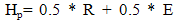 | (2) |
Where R is the internal priority of each process and E is the external priority.Processes with highest Hp are executed first [8].
3. Research Method
3.1. Design of Preemptive Modified Highest Response Ratio Next (PMHRRN)
The required data (burst times and arrival times of processes) will be generated using Poisson distribution. The length of burst time of a process shall be its external priority while its internal priority shall be determined by the response ratio of each process in the ready queue. Response ratio, R and hybrid priority, Hp are computed using equations (1) and (2) respectively.Processes with highest hybrid priority, Hp, will be executed next. After the execution of a burst time, a running process may be preempted if there is another process with a higher hybrid priority. In the event where multiple processes turn up with the highest hybrid priority, the system shall select the process with the earliest arrival time among those processes and then preempt the current running process. If the current running process turns out to be the process with the highest hybrid priority, it continues to run until a process with a higher hybrid priority is found.
3.2. PMHRRN Algorithm
1. Start2. Initialize AWT = 0, ATAT = 0, ART = 03. Processes arrive at the ready queue, RQ.4. Processes in RQ are sorted and assigned priority 5. Hybrid priority, Hp = 0.5R + 0.5E6. Are there multiple processes with highest Hp?If yes, did processes with same highest Hp arrive at same time? If yes, Pi = any process with highest Hp,Else Pi = process with earliest arrival time among the processes Else, Pi = process with highest hybrid priority, Hp7. Pi executes a burst time8. Is RBT [Pi] = 0?If yes, process Pi leaves RQ, calculate WT, R, and TAT of Pi , go to 9 Else go to 49. Is RQ = null?If yes, calculate AWT, ART, ATAT of all processes, go to 10 Else go to 4.10. STOP
3.3. Results and Discussion
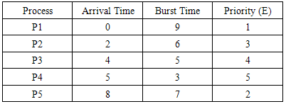
Assumptions of the model are;1. All experiments are performed in a uniprocessor environment.2. All processes are independent of each other.3. Attributes such as burst times and arrival times are known prior to submission of process.4. All processes are CPU bound.Table 1. Data set of five processes
 |
| |
|
Using the data in Table 1, we shall compute the Average Turnaround Time (ATAT), Average Waiting Time (AWT) and Average Response Time (ART) for a set of five processes. The range of burst time used is 0-10.
3.3.1. HRRN
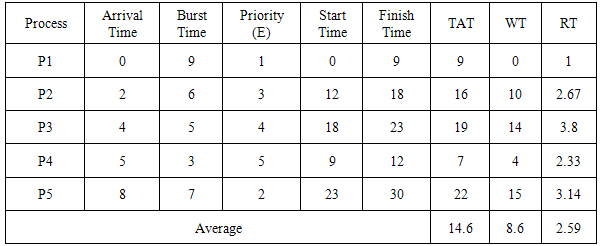
The response ratio, R, of each process is computed and the process with the highest response ratio is assigned the CPU. At time t=0, process P1 is considered for execution (as it is the only available process) and runs to completion for 9 time units and terminates. At time t=9, all the other processes (P2, P3, P4 and P5) have arrived. Notice that each process has waited for some time units while process P1 was running. Process P2 has waited for 7 time units, process P3 has waited for 5 time units, process P4 has waited for 4 time units and process P5 has waited for 1 time unit. The response ratio, R, is computed for processes P2, P3, P4 and P5 using the waiting time of each process and their corresponding burst time as shown in Table 1.P2: R = (7+6)/6 = 2.167P3: R = (5+5)/5 = 2P4: R = (4+3)/3 = 2.333P5: R = (1+7)/7 = 1.143Process P4 has the highest response ratio, R, and as a result runs for 3 time units and terminates.At time t=12, Processes P2, P3 and P5 are available. Notice that each process has waited for some time units while processes P1 and P4 were running. Process P2 has waited for (7+3) time units, process P3 has waited for (5+3) time units and process P5 has waited for (1+3) time units. The response ratio, R, is computed for processes P2, P3 and P5 using the waiting time of each process and their corresponding burst time as shown in Table 1.P2: R = (10+6)/6 = 2.67P3: R = (8+5)/5 = 2.6P5: R = (4+7)/7 = 1.57Process P2 has the highest response ratio, R, runs for 6 time units and terminates. At time t=18, Processes P3 and P5 are available. Notice that each process has waited for some time units while processes P1, P2 and P4 were running. Process P3 has waited for (5+3+6) time units and process P5 has waited for (1+3+6) time units. The response ratio, R, is computed for processes P3 and P5 using the waiting time of each process and their corresponding burst time as shown in Table 1.P3: RR = (14+5)/5 = 3.8P5: RR = (10+7)/7 = 2.43Process P3 has the highest response ratio, R, runs for 5 time units and terminates.At time t=23, Process P5 is the only process available. Notice that process P5 has waited for some time units while processes P1, P2, P3 and P4 were running. Process P5 has waited for (1+3+6+5) time units.Process P5 runs to completion for 7 time units and terminates. Table 2 summarizes the result. Table 2. Summary of HRRN result
 |
| |
|
3.3.2. MHRRN
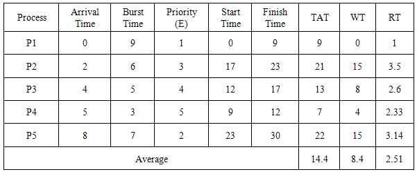
The hybrid priority, Hp, is computed using equation (2). Using the information in Table 1, the MHRRN algorithm is demonstrated as follows;At time t = 0, only process P1 is available, so P1 is considered for execution. Process P1 runs to completion for 9 time units and leaves the queue as the system is NOT preemptive. At time t = 9, processes P2, P3, P4 and P5 have arrived and hybrid priority, Hp is computed as follows:P2: R = (7+6)/6 = 2.167;Hp = 0.5(2.167) + 0.5(3) = 2.58P3: R = (5+5)/5 = 2;Hp = 0.5(2) + 0.5(4) = 3P4: R = (4+3)/3 = 2.333;Hp = 0.5(2.333) + 0.5(5) = 3.67P5: R = (1+7)/7 = 1.143;Hp = 0.5(1.143) + 0.5(2) = 1.57Notice that the response ratio, R, of each process is first computed and the result used as the internal priority in the computation of the hybrid priority, Hp, of that process. P4 has the highest hybrid priority, Hp, runs for 3 time units and leaves the queue.At time t = 12, processes P2, P3 and P5 are available. The hybrid priority, Hp, of each process is computed as follows:P2: R = (10+6)/6 = 2.67; Hp = 0.5(2.67) + 0.5(3) = 2.83P3: R = (8+5)/5 = 2.6; Hp = 0.5(3.3) + 0.5(4) = 3.3P5: R = (4+7)/7 = 1.57; Hp = 0.5(1.57) + 0.5(2) = 1.79Process P3 has the highest hybrid priority, Hp, runs for 5 time units and leaves the queue.At time t=17, processes P2 and P5 are available. The hybrid priority, Hp, of each process is computed as follows:P2: R = (15+6)/6 = 3.5; Hp = 0.5(3.5) + 0.5(3) = 3.25P5: R = (9+7)/7 = 2.29; Hp = 0.5(2.29) + 0.5(2) = 2.143Process P2 has the highest hybrid priority, Hp, runs for 6 time units and leaves the queue.At time t=23, only process P5 is available. Process P5 runs for 7 time units and leaves the queue. Table 3 summarizes the result.Table 3. Summary of MHRRN result
 |
| |
|
3.3.3. PMHRRN
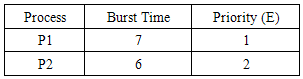
The proposed algorithm, PMHRRN, is a preemptive version of MHRRN. Using the information in Table 1, the PMHRRN algorithm is demonstrated. At time t = 0, only process P1 is available and runs for 2 time units. Note that process P1 runs for 2 time units because it is the only process available for that time period.At time, t = 2, processes P1 and P2 are available. Their priorities are determined as shown in Table 4 and their hybrid priority, Hp, is computed. Note that the longer the burst time of the process, the lower the value of the priority of the process. The burst time of each process is also updated (as shown in Table 4) to indicate the remaining burst time of the process which is used in computing the response ratio (internal priority) of the process.P1: R = (0+7) /7 = 1; Hp = 0.5(1) + 0.5(1) = 1P2: R = (0+6)/6 = 1; Hp = 0.5(1) + 0.5(2) = 1.5Table 4. Process state at t=2
 |
| |
|
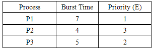
Process P2 has the highest hybrid priority, Hp. P1 is therefore pre-empted and P2 runs for 2 time units. Note that process P2 runs for 2 time units because after the execution of a burst time, when the hybrid priority is recomputed, it turns out to be the process with the highest value.At time t = 4, processes P1, P2 and P3 are available. Their priorities are determined as shown in Table 5 and their hybrid priority, Hp, is computed. The burst time of each process is also updated to indicate the remaining burst time of the process which is used in computing the response ratio (internal priority) of the process.P1: R= (2+7)/7 = 1.285; Hp= 0.5(1.285) + 0.5(1) = 1.143P2: R= (0+4)/4 = 1; Hp= 0.5(1) + 0.5(3) = 2P3: R= (0+5)/5 = 1; Hp= 0.5(1) + 0.5(2) = 1.5Table 5. Process state at t=4
 |
| |
|
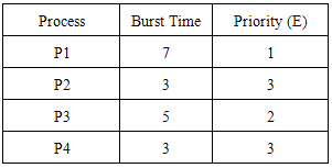
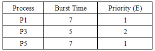
Process P2 has the highest hybrid priority, Hp and so runs for 1 time unit.At time, t = 5, processes P1, P2, P3 and P4 are available. Their priorities are determined as shown in Table 6 and their hybrid priority, Hp, is computed.P1: R = (3+7)/7 = 1.43; Hp= 0.5(1.43) + 0.5(1) = 1.2P2: R = (0+3)/3 = 1; Hp= 0.5(1) + 0.5(3) = 2P3: R = (1+5)/5 = 1.2; Hp= 0.5(1.2) + 0.5(2) = 1.6P4: R = (0+3)/3 = 1; Hp= 0.5(1) + 0.5(3) = 2Table 6. Process state at t=5
 |
| |
|
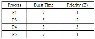
Processes P2 and P4 have the highest hybrid priority, Hp, but process P2 runs for 3 time units because it arrived earlier than P4. It then leaves the queue. Note that process P2 runs for 3 more time units because after the execution of a burst time, when the hybrid priority is recomputed, it turns out to be the process with the highest value.At time, t = 8, processes P1, P3, P4 and P5 are available. Their priorities are determined as shown in Table 7 and their hybrid priority, Hp, is computed. P1: R = (6+7)/7 = 1.86; Hp= 0.5(1.86) + 0.5(1) = 1.423P3: R = (4+5)/5 = 1.8; Hp= 0.5(1.8) + 0.5(2) = 1.9P4: R = (1+3)/3 = 1.333; Hp= 0.5(1.333) + 0.5(3) = 2.167P5: R = (0+7)/7 = 1; Hp= 0.5(1) + 0.5(1) = 1Table 7. Process state at t=8
 |
| |
|
Process P4 has the highest hybrid priority, Hp, and runs for 3 time units and leaves the queue. Note that process P4 runs for 3 time units because after the execution of a burst time, when the hybrid priority is recomputed, it turns out to be the process with the highest value.At time, t = 11, processes P1, P3 and P5 are available. Their priorities are determined as shown in Table 8 and their hybrid priority, Hp, is computed. P1: R = (9+7)/7 = 2.29; Hp= 0.5(2.29) + 0.5(1) = 1.643P3: R = (7+5)/5 = 2.4; Hp= 0.5(2.4) + 0.5(2) = 2.2P5: R = (3+7)/7 = 1.429; Hp= 0.5(1.429) + 0.5(1) = 1.214Table 8. Process state at t=11
 |
| |
|
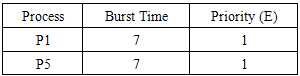
Process P3 has the highest hybrid priority, Hp, runs for 5 time units and leaves the queue.At time, t = 16, processes P1 and P5 are available. Their priorities are determined as shown in Table 9 and their hybrid priority, Hp, is computed.P1: R = (14+7)/7 = 3; Hp= 0.5(3) + 0.5(1) = 2P5: R = (8+7)/7 = 2.143; Hp= 0.5(2.143) + 0.5(1) = 1.57Table 9. Process state at t=16
 |
| |
|
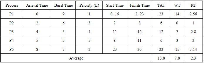
Process P1 has the highest hybrid priority, Hp, runs for 7 time units and leaves the queue. At time t=23, only process P5 is available. P5 runs for 7 time units and leaves the queue. Table 10 summarizes the result.Table 10. Summary of PMHRRN result
 |
| |
|
Figure 1 shows the comparison of parameters studied for HRRN, MHRRN and PMHRRN algorithms based on Table 1.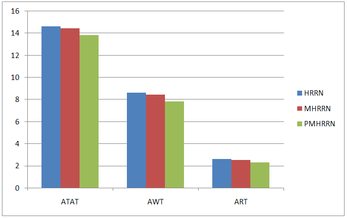 | Figure 1. Comparing parameters for HRRN, MHRRN and PMHRRN |
3.4. Comparing Existing Scheduling Algorithms with PMHRRN
To study the performance of PMHRRN, a system was developed to generate the data used and to compute the results for large sets of data for HRRN, MHRRN and the proposed PMHRRN algorithms. Figure 2 shows the summary of results obtained for a one-time run of 1000 processes with burst range of 1-1200. Table 11 shows a summary of results obtained for ATAT, AWT and ART for 1000 processes with a burst range of 1-1200 run 10 different times.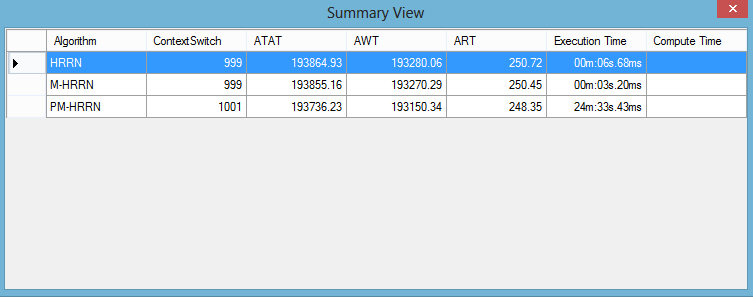 | Figure 2. Screen shot of a one-time run of1000 processes with burst range of 1-1200 |
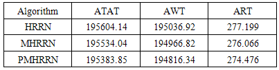
Table 11. A comparison of PMHRRN, MHRRN and HRRN
 |
| |
|
Based on the research, the following is found in terms of performance metrics studied;Response TimeWhile MHRRN performs better than HRRN by 0.41%, PMHRRN performs better than MHRRN by 0.58% and subsequently performs better than HRRN by 0.98%Waiting TimeWhile MHRRN performs better than HRRN by 0.04%, PMHRRN performs better than MHRRN by 0.08% and subsequently performs better than HRRN by 0.11%Turnaround TimeWhile MHRRN performs better than HRRN by 0.04%, PMHRRN performs better than MHRRN by 0.08% and subsequently performs better than HRRN by 0.11%However, as is common to every preemptive algorithm, the major drawback of this scheduling algorithm is time spent in context-switching.
4. Conclusions
The aim of the research was to study the effect of preemption on MHRRN, anon-preemptive algorithm that incorporated both internal and external priorities to determine which process gets the CPU.Upon successful completion of the study, it was found that response times, waiting times and turnaround times of processes in a uniprocessor are found to be minimized with the introduction of preemption on the MHRRN algorithm. Users and designers of operating systems will find PMHRRN algorithm helpful in addressing the issue of starvation, inclusion of external priority and response times especially in interactive systems since the parameters studied have been minimized and as a result, users in the system can be maximized. The proposed algorithm is found to be better than MHRRN in terms of ATAT, AWT and ART.In future, the proposed scheduling algorithm shall be applied on tasks that have dependencies among each other and performance of the proposed algorithm shall be studied in real time applications where tasks have priorities and deadline constraints.
References
| [1] | A. Silberchatz, P. B. Galvin and G. Gagne. Operating System Concepts. 7th ed., John Wiley & Sons. Hoboken, USA. 2005. |
| [2] | J. Patel and A. K. Solanki. “Performance Evaluation of CPU Scheduling by Using Hybrid Approach,” International Journal of Engineering Research & Technology (IJERT) ., 1 (4), 1-8, June 2012. |
| [3] | W. Stallings. Operating Systems: Internals and Design Principles.7th ed., Prentice Hall, USA. 2012. |
| [4] | E. O. Oyetunji and E. Oluleye. “Performance Assessment of Some CPU Scheduling Algorithms,” Research Journal of Information Technology , 1 (1), 22-26, 2009. |
| [5] | M. Abur, A. Mohammed, S. Danjuma,S. Abdullahi S. “A Critical Simulation of CPU Scheduling Algorithm using Exponential Distribution,” International Journal of Computer Science Issues , 8 (6), 201-206, 2011. |
| [6] | J. Niu. http://www.sci.brooklyn.cuny.edu/~jniu/teaching/csc33200/files/1201-UniprocessorScheduling.pdf. Retrieved August 26, 2012. |
| [7] | S. S. Monemi. http://www.csupomona.edu/~carich/classes/cs499/201001/notes/os_fundamentals.pdf. Retrieved April 10, 2013. |
| [8] | S. Varma. “Design of Modified HRRN Scheduling Algorithm for priority systems Using Hybrid Priority scheme,” Journal of Telematics and Informatics (JTI) , 1 (1), 14-19, 2013. |
| [9] | H. S. Behera, B. K. Swain, A. K. Parida, G. Sahu. (2012). “A New Proposed Round Robin with Highest Response Ratio Next (RRHRRN) Scheduling Algorithm for Soft Real Time Systems,” International Journal of Engineering and Advanced Technology , 1 (3), 2012. |
 Abstract
 Reference
 Full-Text PDF
 Full-text HTML