1. Introduction

The ongoing advancements in wireless technology have allowed for many different devices (old and new) to communicate in a wireless network at a declining cost. While some of these networks may consist purely of stationary devices, mobility is the primary advantage of wireless communication. Thus the underlying mechanisms that dictate how a packet is sent from one device to another should reflect not only our understanding of how wireless mobile devices operate, but also our desire for optimal performance. The representation of networks as geometrical graphs provides the foundation for ingenuity in routing protocols. Graphs provide insight into both the optimal aspects of a routing algorithm as well as its limitations. To this end, a thorough examination of several routing algorithms along with their inherent structures and optimality aspects will be presented, beginning with the classical approach in static networks and ending with methods used in homogenous wireless networks.

2. Classical Approaches

While it will be shown that the following static routing algorithms are not appropriate for wireless networks in general, the underlying methods and objectives provide the foundation to which several effective routing protocols are based on[1].

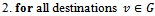
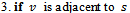
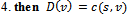
2.1. Link-State Protocol: Dijkstra’s Algorithm

The algorithm presented below produces the shortest path from a source to all possible destinations on a directed graph with non-negative edge weights . Its implementation in networking is known as a link-state algorithm[2, 3]. Let denote the number of nodes in the graph. Let be the total weight of the shortest path from the source to destination . Let be the cost of routing from to (i.e., the sum of all edge weights along the path from to . Finally, let contain the vertices in whose shortest paths have been determined.

Algorithm

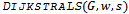Input: a graph (represented by an adjacency list), non-negative edge weights , and source .

Output: weight of shortest path from source to all destinations .

The structure of the above algorithm comes from[2], while a more detailed analysis of its functionality and correctness is outlined in[3]. Lines 6 through 9 are known as relaxing an edge. A total of edges are relaxed, each requiring computations, which results in an overall complexity of . The implementation of a binary heap for the priority queue improves the relaxation computation to and thus the overall complexity to .

Regardless, the implementation of link-state protocols generally requires global state information from the graph. That is, the topology and link-costs are known to every node, which culminates in one exhaustive routing table that is maintained between all nodes. Hence a small change in the topology of the system can propagate into large errors in the routing table. Even with the available global state information, routing loops can still occur; for instance when two nodes and attempt to route through each other to get to a destination . An example of this event will be provided in the next section, as the directed distance vector routing protocol is also sensitive to changes in topology. Thus the use of Dijkstra’s algorithm in wireless ad hoc networks is ill suited due to its static nature, time-complexity, and the overhead requirements it imposes on a network by requiring global state information.

2.2. Directed Distance Protocol: The Bellman-Ford Algorithm

The directed distance-vector routing protocol is nearly identical to the Bellman-Ford algorithm – but with one modification: the relaxation phase uses an infinite while loop in order to achieve a quiescent state that responds to link-cost changes or updated distance vectors[2].

A major distinction between link-sate and directed distance-vector routing algorithms is the amount of information that is available to a given node in a network. The algorithm below uses localized information of a source to calculate the distance vector to each of its neighbours. Once each node has calculated its distance-vector, it is broadcasted to each of their respective neighbours. The result is a minimum weight-spanning tree.

Algorithm

Input: a graph (represented by an adjacency list), edge weights , and source .

Output: weight of shortest path from source to all destinations .

7. while (there exists a link cost change or updated distance vector to some adjacent )

9. do: for all ,

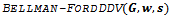
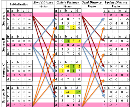
Figure 1 illustrates how the Bellman-Ford algorithm produces the shortest path in the given graph with A as the source. Figure 2 exemplifies the distributive and asynchronous nature of the algorithm where each node maintains its own routing table and sends updated distance vectors to neighbouring nodes.

Note that the purpose of lines 14 to 16 is to check for negative weight cycles within the graph. This may be unnecessary if all edge weights are non-negative, but depending on what the routing costs are representing, negative weights may be unavoidable. For instance, they might signify the load carried or removed from a packet as it travels from a source to a destination. It is simply one of many preventative measures against routing loops. Unfortunately, the Bellman-Ford algorithm can converge very slowly, and despite its ability to accept changes in topology it is prone to routing loops. An example of how a link-cost change can result in a routing loop is shown in Figure 3.[2]

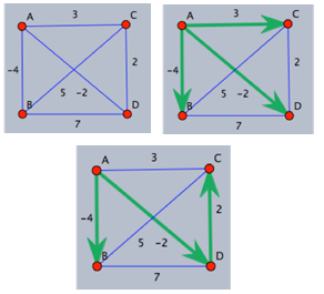Figure 1. Bellman-Ford algorithm applied to the graph on nodes with as the source. The green arrows represent the shortest path from to all other nodes. The change in shortest path reflects the iterative updates in distance vectors

Figure 2. Routing tables associated with the graph in Figure 1. Arrows indicate the forwarding of distance vectors to adjacent vertices. Highlighted cells indicate the detection of new shortest paths derived from recently updated distance vectors

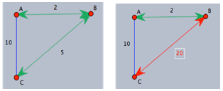Figure 3. Example of how a link-cost change can result in a routing loop

In the first picture of Figure 3, the shortest path has already been determined between nodes, A, B and C. The problem arises when the link cost between nodes B and C changes from 5 to 20. At this moment, B detects the link-cost change and updates its distance vector accordingly to route through A to get to C. But A is not aware of the link-cost change and will continue to route through B to get to C which results in a routing loop between A and B. However, through continually updating their distance vectors, A will eventually route to C directly, terminating the routing loop. This phenomenon is known as the count-to-infinity problem[2]. Adding poisoned reverse is a technique designed to counteract this issue and can be applied to the example in Figure 3 in the following way: since the link-cost change results in B attempting to route through A to get to C, B will broadcast its cost of routing to C as . When A receives the updated distance vector from B, it will now believe that a direct path from B to C does not exist and will therefore route to C directly (as it would have all along if global state information was available).

While localized information certainly decreases the overhead costs of routing protocols, it enables errors to propagate from node to node. Despite the existence of preventative measures such as adding poisoned reverse, Dijkstra's algorithm and the Bellman-Ford algorithm are neither robust nor computationally efficient enough to handle the dynamic nature of wireless ad hoc networks. In order to formulate routing protocols that are appropriate for these purposes, desirable structures will be analysed next.

3. Structures of Wireless Ad Hoc Networks

The remainder of the algorithms to be presented are known to work in planar, connected, unit distance wireless graphs. First, a justification for modeling wireless ad-hoc networks in unit distance graphs will be outlined, followed by localized methods to extract planar sub graphs.

3.1. Unit Distance Wireless Graphs

Let be a set of points in the Euclidean plane. The unit distance wireless graph of contains all points, and edges such that the distance between and is within 1 unit 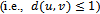[4]. An example of a on a set of 6 points is illustrated in Figure 4.

The reasoning behind using to model wireless networks stems from the concept of broadcast ranges. That is, wireless devices are limited in their ability to communicate with other devices in accordance to their broadcast range. In the , all broadcast ranges are assumed to be uniform, hence can send a packet directly to if and only if is contained within the circle of radius 1 centered at .

Finally, it is entirely reasonable to assume that a wireless device has knowledge of its co-ordinates due to the wide use of Global Positioning Systems.

3.2. Gabriel Graphs

Consider a set of points in the Euclidean plane . The Gabriel circle of two points is defined as the circle that passes through both points and has the segment as a diameter, with the condition that no other point from lies within .

Figure 4. of a set of 6 points: . Each circle has a radius of 1 unit

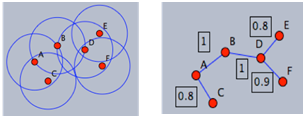
The Gabriel graph of, , consists of all points and edges such that exists[5]. Figure 5 demonstrates the construction of the Gabriel graph on 3 points.

Figure 5. Gabriel Graph of a set of 3 points:

To show that the Gabriel graph is planar we will first assume the opposite and then arrive at a contradiction.

Suppose that there exists a set of points such that the Gabriel graph is non-planar. Then there exists at least one edge intersection between two edges and . Since is a Gabriel edge it follows that neither nor lies inside . Then regardless of the position of or outside of, the circle will contain at least one of the points or . But then cannot be a Gabriel edge, which contradicts the supposition. Therefore, the Gabriel graph on a set of points is always planar. Figure 6 illustrates the proof of the Gabriel graph’s planarity.

Finally, given a connected on a set of points , the intersection of and results in a connected planar subgraph [5].

To prove the connectedness of , suppose that is connected and is disconnected.

Then there exists points such that they are adjacent in but not adjacent in . This necessitates the existence of a third point such that lies within the Gabriel circle . But then and . Hence there are edges and resulting in a path from to in (which contradicts the above supposition). Therefore if is connected, then is connected as well[5].

It follows that a connected planar subgraph can be extracted from any connected by having each node in the graph check for the existence of Gabriel circles between itself and its neighbours. Thus, there exists a localized method to extract planar subgraphs which can be accomplished for each point in time, where is the number of neighbouring nodes to [5].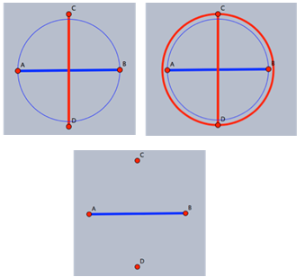

Figure 6. Planarity of the Gabriel graph on a set of 4 points:

3.3. Delaunay Graphs

The Delaunay graph is an excellent structure to have within networks as it contains every Gabriel edge. Although the relative neighbourhood graph will not be discussed in this paper, it is worth mentioning that the Gabriel graph contains the relative neighbourhood graph as a subgraph, and the relative neighbourhood graph contains the minimum spanning tree as a subgraph. Hence the Delaunay graph contains many valuable structures as subgraphs. Finally the connectedness and planarity of the Delaunay graph and all its subgraphs can be derived from the idea of “forbidden zones” (e.g., the Gabriel circle between any two points is a forbidden zone for any other point) and using the relationships between the above-mentioned structures. However, this is beyond the scope of this paper and will be left for the interested reader as an exercise.

Before defining the Delaunay graph of a set of points , we must define the convex hull. The convex hull of a set of points is the smallest enclosing polygon comprising of all points with the condition that every line is completely contained within [6].

The Delaunay graph partitions the convex hull into disjoint triangles with the condition that the circumcircle of each triangle does not contain any other point in.

is uniquely defined if no 4 points are co-circular[5].

is dual to the Voronoi diagram which divides the plane into disjoint regions. Each region is defined by a point such that anything within the region is closer to than any other point . The Voronoi diagram can be computed in time; therefore, due to its duality, can be calculated in the same time[6].

It has been suggested in[5] to force a wireless network to contain the Delaunay graph by either increasing the transmission rates of the wireless devices or by deploying more radio stations.

4. Routing in Wireless Ad-Hoc Networks

There are many approaches to routing in wireless ad-hoc networks. An absolute necessity in employable routing protocols is the guaranteed delivery of packets to their destination. Compass Routing and Face Routing can guarantee delivery in certain geometric structures as outlined below.

4.1. Compass Routing

Given a planar on a set of points in the Euclidean plane, suppose that a point intends to send a packet to a destination (Note if is non-planar, then compute ). The forwarding packet must maintain the location of its: current position , destination, and all nodes adjacent to .

Algorithm

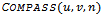Input: the location of a packet’s: current position , destination , and adjacent nodes .

Output: arrival of packet at its destination

1. Forward packet to neighbour such that the slope of is closest to amongst all

2. if

3. then report arrival of packet at destination, break

4. else

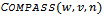Figure 7 illustrates how this recursive algorithm would proceed on a graph of 8 nodes. Nevertheless, Compass routing is known to work on Delaunay graphs that are uniquely defined, but is still prone to routing loops in graphs with low convexity, and can even fail in convex graphs[5].

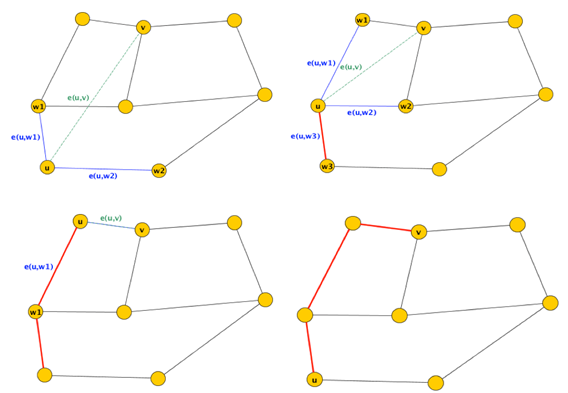Figure 7. Forwarding of a packet from to its destination using Compass routing in the given graph of 8 nodes

Randomized compass routing guarantees delivery in convex subdivisions by modifying the above algorithm to forward packets randomly to adjacent nodes where and are the neighbours of that minimize the clockwise and counter-clockwise angle between all and . The packet could theoretically take a very long time to arrive at its destination but in practice, randomized compass routing performs well[5].

4.2. Face Routing

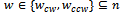
Just as the name suggests, face routing considers the disjoint regions induced on the plane by the edges of the on a set of points, wherein some edges are considered to appear twice (namely the edge shared between two traversed faces). In addition to a distance (initially set to 0), a packet must maintain the locations of: its origin, an intermediate point , the destination , and the previous two nodes visited and. This last requirement helps prevent the occurrence of routing loops[4].

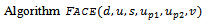Input: distance (initially set to 0), and the locations of: its origin , a point (initially set to), the destination , and the previous two nodes visited and (initially set to null)

Output: arrival of packet to its destination

1. determine the face , incident to that is intersected by the line

2. begin the traversal of , updating and after each edge traversal

3. if packet arrives at

4. then report arrival of packet at destination

6. else upon intersecting the line, calculate the distance from u to this intersection point

9. upon arriving back at traverse until has been reached

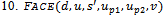Refer to Figure 8 for a simulation of face routing on the given graph of 17 nodes.

Out of all the algorithms presented, face routing is by far the most robust as it is known to work on all planar networks. Due to the constant amount of memory of the packet, the algorithm handles changes in topology very well. For instance if one of the nodes along the path from to stops transmitting its signal, the packet and its forwarding method is unaffected unless the packet resides at the failed node in question. If this is the case then the packet of will not reach its destination since only one copy of the packet is forwarded from node to node. Aside from this scenario, a packet is also subject to routing loops if a node along the path from to continually fails and recovers during a face traversal; but this is a highly degenerate case. Finally, each of the edges of a given face is traversed at most twice[4].

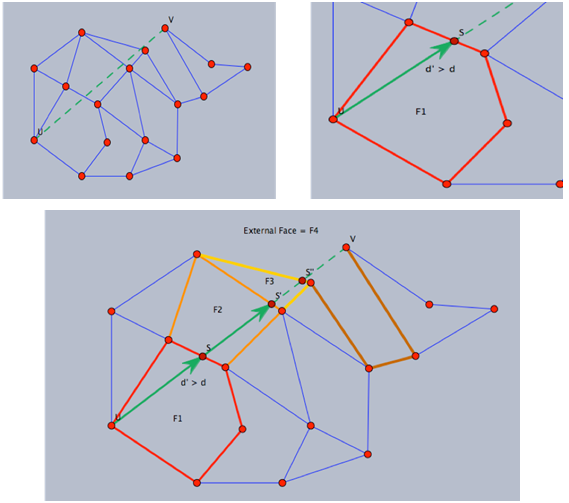Figure 8. Face routing on a graph of 17 nodes. Non-blue edges indicate an edge traversal. In this scenario, 4 faces are traversed in total (including the external face) in order to deliver a packet from to

5. Conclusions

At first glance it would appear that the link-state and distance-vector routing protocols are ill suited for wireless ad-hoc networks, but the majority of heuristic protocols used are largely influenced by their methodologies[1]. What is highly undesirable of these methods is the overhead costs associated with maintaining routing table(s).

The unit distance wireless graph is a good representation of wireless ad hoc networks in which the wireless devices all have a uniform broadcast range. Of course, there are many cases in which broadcast ranges are not uniform, and there are often environmental factors that can inhibit a transmitter’s signal strength. However this model provides the foundation to which compass routing and more importantly face routing can guarantee delivery.

It was suggested in[4] that since nodes within a unit distance wireless graph generally have relatively few adjacent nodes, the greedy quadratic time algorithms are better suited for determining incident edges, as their implementation is simpler. However, the robustness and scalability of face routing is undeniable and should at least be employed as an alternative routing protocol when routing loops persist within a system.

Many other on-demand routing protocols like face routing and compass routing require methods to extract planar subgraphs. This paper discussed only the use of the intersection of the Gabriel graph and the unit distance wireless graph as an alternative to the greedy approach. The relative neighbourhood graph is another nice geometric structure that can be derived in the same amount of time and is equally useful in the formation of localized routing algorithms[2, 6].

ACKNOWLEDGEMENTS

Dr. Vassilev’s research is supported by NSERC Discovery Grant.