Dominik Strzałka
Department of Distributed Systems, Rzeszow University of Technology, Al. Powstańców Warszawy, 2, 35-959, Rzeszów, Poland
Correspondence to: Dominik Strzałka , Department of Distributed Systems, Rzeszow University of Technology, Al. Powstańców Warszawy, 2, 35-959, Rzeszów, Poland.
| Email: |  |
Copyright © 2012 Scientific & Academic Publishing. All Rights Reserved.
Abstract
Many different measures were proposed to describe the problem of possible software complexity - the number of lines of code sometimes referred as a source lines of code (SLOC), Halstead’s volume V, McCabe cyclomatic number V(G), among others. However, any of them doesn’t take into account the possible fractal properties of software source code emerging from development process. The main aim of this paper is to show that in the case of successive Linux OS kernels fractal self-organization of the system can be seen. This is done in the relation to: (i) the analysis of rate of growth for number of files and source lines of Linux kernels code, (ii) by the presentation of some visualizations indicating self-similar graphical structure of OS kernels, (iii) by the calculations of fractal dimensions Db basing on box dimension method. Basing on obtained results it can be assumed that: (i) calculated rate of growth in the case of lines and files in the simplest approach can be approximated by the polynomial with degree 2 with R = 0.96 and R = 0.94 respectively, (ii) this system becomes more and more complex with self-similar structure, (iii) its fractal dimension is still growing. Presented analysis opens new possibilities for description of computer programs in terms of complex systems approach.
Keywords:
Linux Kernel Maps, Fractal Dimension, Emergence, Complex Systems
Cite this paper:
Dominik Strzałka , "Fractal Properties of Linux Kernel Maps", Computer Science and Engineering, Vol. 2 No. 6, 2012, pp. 112-117. doi: 10.5923/j.computer.20120206.05.
1. Introduction
A branch of software metrics that is focused on direct measurement of software attributes is called the software complexity[1]. It can be used to provide a continuous feedback during a software project to help control the development process and to predict the critical information about reliability and maintainability of software systems. There are many different software complexity measures: the number of lines of code sometimes referred as a source lines of code (SLOC), Halstead’s volume V, McCabe cyclomatic number V(G), etc[2]. The most popular one is the number of source lines of code (SLOC). This measure gives the size of software program by counting the number of lines in the text of program’s source code. It helps to predict the amount of effort that would be required to redevelop the program. Line count is usually big, it can even reach 107 lines – see the examples in Table 1. However, this measure has many disadvantages, for example the lack of accountability, the lack of counting standards, the problems with multiple languages, etc. Bill Gates said that[3]: “Measuring programming progress by lines of code is like measuring aircraft building progress by weight”. Despite all that, this quantity is quite often given, because it can help imagine how difficult the development was and how “big” the software is.Table 1 shows information based on data taken from[4,5,6] that presents different operating systems size in millions of SLOC. As it can be seen the most popular operating systems consist of roughly 50 or more millions lines of code. This information gives a clue of how complicated (or maybe complex) the structure of such a system can be, by dint of the possible existence of different dependencies between particular parts of analyzed system. However, it doesn’t say anything about the nature of this dependencies and possible patterns that can emerge. It is quite hard to imagine how complicated (complex) can be the structure of operating system due to many reasons. Company secrets concealing the details of given operating system functionality is one of them – there is no access to the source code or detailed documentation that will be helpful in such investigations. Obviously, because nowadays operating systems consist of millions lines of source code it is almost impossible to analyze it without “creative” methods of analysis.But in some cases there is a possibility to have the access to the operating system source code and the most interesting example here is Linux OS. This system was introduced by Linus Torvalds in 1991. At the beginning, his work was treated rather as a some kind of “software toy”, but now it is assumed that is used by about 30 mln of people. This development phenomenon is very interesting itself because of many reasons. One of them will be presented in this paper, where we would like to focus on self-organized fractal properties of Linux kernel maps visualizations.| Table 1. Lines of code in different operating systems |
| | Operating System | SLOC (Milions) | | Windows NT 1.0 (known as 3.1) | 4-5 | | Windows NT 2.0 (known as 3.5) | 7-8 | | Windows NT 3.0 (known as 3.51) | 9-10 | | Windows NT 4.0 (known as 4.0) | 11-12 | | Windows NT 5.0 (known as Windows 2000) | ≥29 | | Windows NT 5.1 (known as Windows XP) | 40 | | Windows NT 5.2 (known as Windows Server 2003) | 50 | | Windows NT 6.0 (known as Windows Vista) | > 50 | | Windows NT 6.1 (known as Windows 7 and Win. Server 2008) | ??? |
|
|
The paper consists of 5 sections. After the introduction, in Section 2, a wide context of systems self-organization and its relation to computer science is presented, as a basic concept in the case of complex systems. Section 3 presents analysis of Linux kernel development basing on lines of code and the number of files in successive versions. Analysis of fractal dimension for generated self-similar maps is presented in Section 4. Section 5 closes the paper with conclusions.
2. Systems Self-organization
A self-organization is one of the most amazing properties in the case of many complex systems. It can be considered as a process in which the internal organization of a system (usually it’s an open system), increases in complexity without management by an outside source. Systems that self-organize typically display many emergent properties. The term self-organization was used for the first time by I. Kant in his “Critique of Judgment”, however its introduction to contemporary science was done in 1947 by the psychiatrist and engineer W. R. Ashby[8]. Then it was taken up by the cyberneticians (H. von Foerster, G. Pask, S. Beer and N. Wiener) in[9], however it didn’t become common in the scientific literature (except in the field of complex systems theory) before the 1970s and especially after 1977 when I. Prigogine (a Nobel Prize Laureate) showed the thermodynamic concept of self-organization.In the case of mathematics and computer science this phenomenon is usually connected with the ideas of cellular automata, graphs (especially in complex networks, like ”small worlds” and scale-free networks), and some instances of evolutionary computation and artificial life. In the field of multi-agent systems, the problem of engineering such systems that will present self-organized behavior is very active research area. This paper shows that there are also other fields where the self-organization can appear. Cooperation of many programmers (sometimes totally independent) in development of software is a great example here.A question arises: how self-organization can be uncovered? And when we can say, with full responsibility: “this system has self-organizing properties”? The answers are from one hand simple, but from the other not, because the self-organized systems display many emergent properties. From one hand we can see its prevalence in the surrounding environment, while form the other we can’t give one pattern or example that will exactly fit to all cases. One of the very interesting examples of self-organized systems are fractals. It is due to the fact that many systems self-organize in self-similar structures (see for example[10]). One of the most commonly known examples of such structures are cauliflowers or more spectacular one – a romanesco. As it is known the fractals are mathematical sets that can’t be directly seen in Nature in the way that they are built (by the recurrence definition with the possibility of infinite number of magnifications that can be done and always will look exactly the same as the whole fractal), however one of the main feature of fractals is the self-similarity property, which is one of the most frequent properties of shapes, systems, things, etc. either natural or -sometimes - human-made. Recalling the famous words of B. Mandelbrot, who in his book[11] wrote that: “Clouds are not spheres, mountains are not cones, coastlines are not circles, and bark is not smooth, nor does lightning travel in a straight line”, we can imagine that the self-similarity property is an inherent feature of many complex systems. But, are the computer systems the complex ones with the self-organized patterns? If we consider the computer systems only as Turing machines implementations we may assume that they are at least complicated systems[12]. However, each such an implementation is the system that has a physical nature not only in the sense that it needs energy for normal work or is built from physical components, but also it is governed by laws and dependencies that have such physical nature. The problem of computer systems complexity was noticed many years ago for example by P. Wegner in 1976 or by M. Gell-Mann in 1987. P. Wegner in[13] wrote that: “When computers were first developed in the 1940’s (...) software costs were less than 5% of hardware costs. (…) In the 1950’s and 60’s hardware costs decreased by a factor of 2 every two or three years and computers were applied to increasingly[number of] systems. (...) to accomplish such tasks[it] may require millions of instructions and millions of data items, (...)[it] has led to a situation where software costs averaged 70% of total system cost in 1973. (...) an important reason for skyrocketing software costs arises from the fact that current large software systems are much more complex (...) than the systems being developed 25 years ago or even ten years ago. It was pointed out by Dijkstra[in 1972] that the structural complexity of a large software system is greater than that of any other system constructed by Man (...)”. M. Gell-Mann argues in[14] that: “(…) chose topics that could be helped along by these huge, big, rapid computers that people were talking about – not only because we can use the machines for modeling, but also because these machines themselves were examples of complex systems”. Thus even if one has a single computer system (as a Turing machine implementation) that isn’t connected to the network, this system can be in many ways considered as a complex one and the self-organization patterns can appear. This view will be presented in details further in the paper using probably most important piece of software – the operating system.
3. Linux Kernel
Let’s start with the short story of Linux. Despite that it can be found very quickly in Internet, we would like to quote what can be read from linux.org[15]: “Linux is an operating system that was initially created as a hobby by a young student, Linus Torvalds, at the University of Helsinki in Finland. Linus had an interest in Minix, a small UNIX system, and decided to develop a system that exceeded the Minix standards. He began his work in 1991 when he released version 0.02 and worked steadily until 1994 when version 1.0 of the Linux Kernel was released. The kernel, at the heart of all Linux systems, is developed and released under the GNU General Public License and its source code is freely available to everyone. It is this kernel that forms the base around which a Linux operating system is developed. There are now literally hundreds of companies and organizations and an equal number of individuals that have released their own versions of operating systems based on the Linux kernel.” 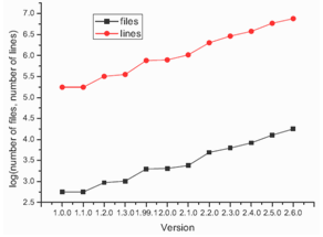 | Figure 1. Number of files and source lines of code for different stable and unstable Linux kernels |
| Table 2. Number of files and source lines of code for different (stable and unstable) Linux kernels |
| | Version | Files | Lines | | 1.0.0 | 561 | 176250 | | 1.1.0 | 559 | 176177 | | 1.2.0 | 936 | 320359 | | 1.3.0 | 1021 | 354718 | | 1.99.1 | 1980 | 764386 | | 2.0.0 | 2048 | 787743 | | 2.1.0 | 2396 | 1040695 | | 2.2.0 | 4910 | 2015857 | | 2.3.0 | 6242 | 2908275 | | 2.4.0 | 8330 | 3783473 | | 2.5.0 | 12727 | 5879352 | | 2.6.0 | 17784 | 7583159 |
|
|
The most important information about Linux is that its code is freely available to everyone thus anyone can develop it. From the beginning it was assumed that Linux source code will be freely available and now this access is based on GNU General Public License. This is the reason why Linux development can be done by many enthusiasts from all over the World. The whole situation (process) can be compared to the river basin behavior: the work that is done by many enthusiast is similar to the rainfalls in river basin while the developed Linux kernel, which emerges as a cumulated work, to the river as a final product of rainfalls in a wide basin. Sometimes the Linux improvements can be very significant (high rainfall) – sometimes they can be very petty (small rainfall); some of the implemented ideas become a significant part of this system, but some aren’t further developed, etc. As it can be seen, the quite short history of Linux isn’t any obstacle in developing of this operating system in a very quick way. The first version of Linux had just a couple of hundreds of lines of code, whereas the latest versions have millions. Details can be found in Table 2. As it can be seen (Fig. 1) Linux growth is very rapid (ordinate represents log values). The quick and unexpected development of Linux OS and the whole Linux community is not only surprising for people who are not well aware of Linux history and its present state but also for scientific community, who started publish many different papers about this phenomenon. As the examples Tuomi or Godfrey papers can be given[20,16]. The last one shows the state of Linux development at the end of 2000. Author assumes that the Linux quick growth can be expressed by the equation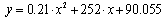 | (1) |
with R2=0.997 where y denotes the size in millions of lines of codes without comments, x denotes days since Linux kernel version 1.0 was released. To show the actual state of Linux kernel development the detailed analysis of numbers of files and lines of code that were added, changed or deleted for each kernel release were prepared, basing on information that can be found in LinuxHQ[21]. It should be noted that Linux kernels are numbered in very interesting way: it is x.y.z. The first number denotes a major release (now it is 2), second it’s minor release and if this number is even it means that this is stable kernel, while the odd number denotes unstable (developed) kernels. The last number is a revision number. Each first stable kernel (i.e. revision 0) is based on latest version of unstable one, i.e., it is released when the whole previous development work has been done, while the unstable kernels can be released when the development of stable kernels hasn’t been finished. For example: the unstable kernel ver. 2.1.0 was released on 30 September 1996, while the latest stable version of stable kernel 2.0.40 was released on 8 February 2001. This explains the structure of two graphs (Fig. 2 and Fig. 3) where the number of files and lines of code for each release of successive Linux kernels (starting from 1.0) is presented. 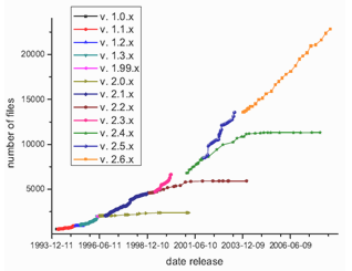 | Figure 2. Number of files in successive stable and unstable Linux kernels according to date of kernel release |
 | Figure 3. Number of source lines of code for successive stable and unstable Linux kernels according to date of kernel release |
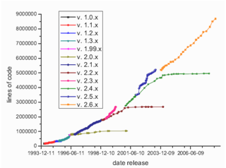
Basing on this information, similarly to the equation (1), the models that express the quick growth of Linux kernels size in the case of lines of code and the number of files were calculated. The calculations were based on all available data points since kernel version 1.0 and for parameters estimation all points were used. In the case of equation (1) the authors didn’t explain how they achieved their results, i.e., did they use all available points data in December 2000 or only those which “fit” to their model –Fig. 2 shows that stable kernels (especially v. 2.0.x, v. 2.2.x or v. 2.4.x) didn't grew as fast as unstable ones starting in similar development points. In the case of files we obtain following model and the variance:  | (2) |
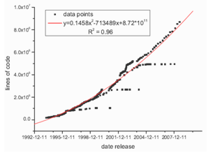
with R2=0.94 while in the case of lines of code it is  | (3) |
with R2=0.96. As it can be seen the comparison of equations (1) and (3) indicates that the obtained results has changed a lot.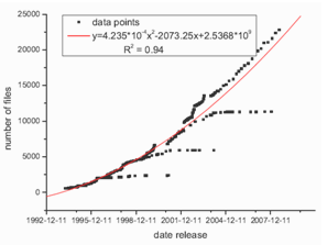 | Figure 4. Polynomial fit (degree 2) of growth of files number for all kernels (stable and unstable) since v. 1.0 |
 | Figure 5. Polynomial fit (degree 2) of growth of source lines of code for all kernels (stable and unstable) since v. 1.0 |
Figs. 4 and Fig. 5 show that kernel v. 2.6.x follows different trend than other stable kernels from 2.x.y family. In this case the growth is very rapid similarly to the unstable kernels. Obvious question appears: why this family of kernels acts this way? Maybe this is connected with the raising functionality of new kernel versions or because of a big number of new hardware solutions that are rather novel and require appropriate drivers. Another reason can be the increasing popularity of Linux itself because it's easy accessible via Internet – nowadays many people have a PC computer with the access to the Internet. This increase can be also caused by the growing number of people who don’t like operating systems from Microsoft or simply by the so far unknown trends. Probably the explanation of this fact isn’t as simple as it seems to be, but this observation is very interesting. This also seems to be in contradiction to the common opinion that maintaining such a big system is extraordinarily difficult and complicated[16]. The whole process obviously needs a lot of time: in the case of latest kernel versions 2.6.x there are 3-4 releases per year, but in the case of previous kernels releases, i.e., 2.4.x and 2.2.x the situation was similar or even “worse” (2-3 releases per year – see[21]).
4. Fractal Properties of Linux Kernel Maps
Information given in Section 3 from one hand can help imagine how the structure of Linux kernel can be complicated (complex), but from the other hand it doesn’t say anything about the real complexity of Linux kernel structure. Graphical visualization can be used to solve this problem. It was done for the first time by Rusty Russell, who introduced The Free Code Graphing Project[19]. Basing on his proposal six visualizations for Linux stable kernels were made i.e. Kernel v. 1.0, v. 1.2, v. 2.0.1, v. 2.2.0, v. 2.4.0, v. 2.6.0 (this paper shows only two of them: Fig. 6 for v. 1.0 and Fig. 7 for v. 2.6.0). 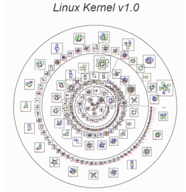 | Figure 6. Visualization of Linux kernel v. 1.0 |
 | Figure 7. Visualization of Linux kernel v. 2.6.0 |
Each visualization represents the inner structure of Linux kernel. It is built from rings that represent the folders used to organize the source code files. The inner ring has all files from the ipc, kernel, lib, mm and init directories (all piled together). The second ring incorporates two segments: the fs/ segment and the net/ segment. The third ring has got one segment per architecture, and the final ring has all drivers piled together. In each ring there are boxes (solid border) that represent the *.c files from the kernel tree. Each box contains smaller boxes (dotted outlines) with colored lines that show three types of functions: static (dark green color), indirect (light green color) and non-static (blue color). The layout of drawing is given as follows: from inner to outer, from smallest to largest, with an iterative spacing increase if there is too much gap in the outer ring. As it can be expected the structures of obtained visualizations from version to version are more and more complicated. However, all the visualizations indicate the existence of self-similarity property, which can be observed in different regions of figures for zoomed parts. It is a very interesting fact that the work that has been done by many programmers during many years as a result can be visualized this way, indicating the existence of some kind of “order” in the whole structure. Because the generated maps indicate possible existence of self-similarity, fractal dimension was calculated using box dimension approach. The box dimension is defined as the exponent Db in the relation  | (4) |
where N(d) is the smallest number of boxes of linear size d necessary to cover a data set of points distributed in a two-dimensional plane. Simple fact acts as basis of this method: for Euclidean objects, the number of boxes necessary to cover a set of points lying on a smooth line is proportional to 1/d, proportional to 1/d2 to cover a set of points evenly distributed on a plane, proportional to 1/d3 to cover a set of points evenly distributed in a space, and so on …, thus the equation (4) defines their dimension by the value of Db exponent (for Euclidean objects this is an integer value). A box dimension can be defined basing on the number of occupied boxes that are placed at any position and orientation, however the number of boxes needed to cover the set should be minimized as much as it is possible. Finding the configuration that minimizes N(d) among all the possible ways to cover the set with boxes of size d proves to be quite difficult computational problem. If the overestimation of N(d) in a box dimension is not a function of scale, which is a plausible conjecture if the set is self-similar, then using boxes in a grid or minimizing N(d) by letting the boxes take any position is bound to give the same result. This is because of power law (such as (4)) behavior - the exponent does not vary if one multiplies N(d) or d by any constant. However, because the assumption not always can be fulfilled in practice, to ensure that the obtained results will be reliable, one can rotate the grid for each box size by some value of degrees and take the minimal value of N(d). In presented analysis the angular increments of rotation were set to 15° Because the equation (4) represents a power law, to calculate the value of Db plots of log(N(d)) on the vertical axis versus log(d) on the horizontal axis were made. The successive points usually follow a straight line with a negative slope that equals Db. There is another problem in this approach - the range of values of d. Trivial results could be expected for very small and very large values of d thus the calculations of the slope were done for two sets of data: all obtained points and for points that lie between 10%-90% of available d values (the extremes were discarded). The obtained results are in Table 3. As it can be seen the latest kernel versions have higher Db dimension than the first ones. | Table 3. Db dimension for visualizations of stable Linux kernels |
| | Kernel | Db | Db (for 80% of points) | | 1.0.0 | 1.407 | 1.386 | | 1.2.0 | 1.436 | 1.423 | | 2.0.0 | 1.455 | 1.461 | | 2.2.0 | 1.536 | 1.553 | | 2.4.0 | 1.587 | 1.612 | | 2.6.0 | 1.629 | 1.661 |
|
|
5. Conclusions
Some interesting properties of open software structure and its development were shown in this paper. Among them one can indicate: quick growth of Linux kernel measured by number of source lines of code and number of used files (in the simplest approach this growth can be approximated by polynomial with degree 2), self-similar visualizations of different stable Linux kernels, calculated box dimension for these visualizations. Because Linux OS is, in many people opinion, independently developed by many enthusiasts all over the world one can imagine that its structure won’t reflect any interesting properties. However, as it turned out this structure shows the existence of system self-organization (Figs. 6 and 7) with self-similar visual patterns. Used box counting method gives calculations for box dimension giving a possibility for description of the complex nature of software systems in terms of fractals. Having this, problems of software evolution can be considered with new metrics and laws, but the proposed approach needs to be developed in future work.Notes
1the difference between complex and complicated systems is quite subtle: the complicated system is a system that has many interdependent elements, but the dependencies between them are governed by well-known deterministic laws (i.e. such systems are rather simple systems), while in the case of complex systems the dependencies between their components are governed by laws that are not necessary well-known. See the details in [7]
References
| [1] | T.J. McCabe, A.H. Watson, Software Complexity, Crosstalk, 12 (1994) 5-–9. |
| [2] | J.K. Nurminen, Using software complexity measures to analyze algorithm – an experiment with the shortest-paths algorithms, Comp. & Op. Res. 30 (2003) 1121–1134. |
| [3] | The Aircraft Working Group: Aircraft’s Role in NextGen, JPDONewsletter,http://www.jpdo.gov/library/newsletter/200806_JPDO_newsletter.pdf, (Access: 10 October 2009). |
| [4] | L. O’Brien, How Many Lines of Code in Windows?, http://www.xhovemont.be/archive/2005/12/07/1072.aspx, Knowing.NET, (Access: 18 January 2008) |
| [5] | J.M. González-Barahona, M.A. Ortuńo Pérez, P. de las Heras Quirós, J.C. González, V.M. Olivera, Counting potatoes: the size of Debian2.2,http://people.debian.org/jgb/debian-counting/counting-potatoes/, debian.org, (Access: 18 January 2010). |
| [6] | G. Robles, DebianCounting,http://libresoft.dat.escet.urjc.es/debian-counting/, (Access: 25 March 2010). |
| [7] | F. Grabowski, D. Strzałka, Simple, Complicated and Complex Systems – The Brief Introduction, 2008 Conference On HSI, 1-2 (2008) 576–579. |
| [8] | W.R. Ashby, Principles of the Self-Organizing Dynamic System, J. of Gen. Psych. 37 (1947) 125–128. |
| [9] | H. von Foerster, G. Pask, S. Beer, H. Wiener, Cybernetics: or Control and Communication in the Animal and the Machine, MIT Press, 1961. |
| [10] | V.N. Smirnov, A.E. Chmel, Self-SimilarityandSelf-Organization of Drifting Ice Cover in the Arctic Basin, Dokl. Earth Sci. 411 (2006) 1249–1252. |
| [11] | B.B. Mandelbrot, Fractal geometry of Nature, Freeman, 1983. |
| [12] | D. Strzałka, Paradigms evolution in computer science, Egitania Sciencia, 6 (2010) 203–220. |
| [13] | P. Wegner, Research paradigms in computer science, Proc. of the 2nd Int. Conf. on Soft. Eng., San Francisco, California, (1976) 322–330. |
| [14] | M. Waldrop, Complexity. The emerging science at the edge of order and chaos, New York, London, Toronto, Sydney, Simon & Schuster Paperbacks, 2008. |
| [15] | http://www.linux.org/info/index.html (Access: 19 March 2009). |
| [16] | M. Godfrey, Q. Tu, Growth, Evolution, and Structural Change in Open Source Software, Proc. of the 4th Int. Work. on Prin. of Soft. Evol., Vienna, Austria (2001) 103–106. |
| [17] | M.M. Lehman, J.F. Ramil, P.D. Wernick, D.E. Perry, W.M. Turski, Metrics and laws of software evolution – the nineties view, Proc. of the 4th Int. Soft. Metr. Symp. (Metrics’97), Albuquerque, NM, 1997. |
| [18] | http://www.oss-watch.ac.uk/resources/gpl.xml#body.1_div.2 (Access: 22 May 2010). |
| [19] | R. Rusel, Free Code GraphicProject,http://fcgp.sourceforge.net/, (Access: 20 January 2010). |
| [20] | I.Tuomi, Internet, Innovation, and Open Source: Actors in the Network, Peer-rewieved J. of the Internet: First Monday, 6, URL:http://firstmonday.org/issues/issue6_1/tuomi/index.html (2001) |
| [21] | http://www.linuxhq.com/kernel/ (Access: 5 September 2009). |
 Abstract
 Reference
 Full-Text PDF
 Full-Text HTML