Aamna Saeed
Department of Computer Science, Military College of Signals, National University of Sciences & Technology, Rawalpindi, Pakistan
Correspondence to: Aamna Saeed , Department of Computer Science, Military College of Signals, National University of Sciences & Technology, Rawalpindi, Pakistan.
| Email: |  |
Copyright © 2012 Scientific & Academic Publishing. All Rights Reserved.
Abstract
High-resolution image mosaics construction is one of the significant topics of research in the fields of computer vision, image processing, and computer graphics. Video mosaics contain enormous valuable information but when analyzing, searching or browsing a video, redundancy between frames creates problem. Therefore it is more suitable to bring together all the frames of a shot into one single image called a mosaic. The idea of Multi-resolution mosaics comes when it is needed to handle large variations in image resolution. As the camera zooms in and zooms out changes in image resolution occur within the video sequence. Some frames which are zoomed in are at higher resolution and contain more detail. If the mosaic image is constructed in low resolution it results in loss of high frequency information in the regions of mosaic that corresponds to high resolution frames. On the other hand if the mosaic image is constructed at the highest resolution it will result in over sampling the low resolution frames. Varying image resolutions can be handled by multi-resolution mosaic data structure Zooming information of each pixel is recorded in a multi resolution data structure. In a multi resolution mosaic user can view the actual zooming information and can distinguish the region with and without zooming information.
Keywords:
Mosaic, Frames, Multi-Resolution, Over Sampling
Cite this paper:
Aamna Saeed , "Multi-Resolution Mosaicing", Computer Science and Engineering, Vol. 2 No. 6, 2012, pp. 101-111. doi: 10.5923/j.computer.20120206.04.
1. Introduction
As information technology develops day by day, video image mosaics are becoming focus of research in image processing, computer vision, photogrammetric fields, and computer graphics[1].Image mosaicing is a famous means of effectively increasing the field of view of a camera by allowing numerous views of the same scene to be gathered into a single image[2].Multi-resolution mosaics are mosaics that handle large variations in image resolution. Changes in image resolution occur within the sequence e.g. as the camera zooms in and zooms out. The zoomed out frame would have to be magnified using some form of pixel replication or interpolation[3].In a video which includes zooming camera motion, all frames are not captured at the same resolution. Frames in which objects are zoomed in usually contain more details. When these frames are registered they need to be resized so that they align on the single coordinate plane of mosaic image The resizing of zoomed images causes loss of spatial information. When the size of an image is reduced a large number of pixels have to be either deleted or overwritten. Consider a video which zooms in on a particular panoramic scene. Although the total number of pixels per image, alsoknown as the resolution is same for all frames of the video but the objects in the zoomed frames would have more detail. All frames of the video sequence have to be mapped to a single reference frame that is the coordinate system of the final mosaic image. Multi-resolution mosaic is a new kind of mosaic that preserves the actual resolution of each object in a video. The information loss during transformations of frames for alignment is overcome. Zooming information of each pixel is recorded in a multi-resolution data structure. In a multi- resolution mosaic user can view the actual zooming information of every object.Image Mosaic technology is very important and efficient to acquire more extensive scenes. Development of digital images becomes more and more prosperous due to fast growth of information technology[4].In literature several techniques have been presented that are robust against illumination variations, moving objects, image rotation and image noise[5]. Researchers have focused on parallax affect and object motion that results in misalignments of frames[6].Proper blending of image features at different resolutions i.e., multi-resolution analysis has been introduced by Su, M.S., et al[7]. Images that are misaligned due to subpixel translation, rotation or shear are difficult to fully re-align. Stitching of such images can result in a mosaic in which discontinuities are clear. Another technique presented by Li, J.S and Randhawa, S provide a method for creation of a seamless mosaic to reduce discontinuities[8].The regions of high resolution which represents the camera’s varying focal length are not necessary to be limited to a single area within the still image. If the camera zoomed in on an area and then panned, there would be a “stripe” of high resolution. If the camera zoomed in and out while panning, there would be several regions of high resolution. For such scenarios L.A Teodosio and W.Bender have presented an approach where mosaic is constructed at the overall highest resolution, scaling the low resolution frames by interpolation[9].Interactive visualization of high-resolution, multi-resolution images in 2D has been addressed by I. Trotts., et al. A method for interactive visualization of multi-resolution image stacks is described. The technique relies on accessing image tiles from multi-resolution image stacks in such a way that, from the observer's view, image tiles all emerge the same size approximately even if they are accessed from diverse tiers within the images comprising the stack. This technique enables efficient navigation of high resolution image stacks[10].The techniques described so far have used a single-resolution compositing surface to blend all of the images together. In many applications, it may be required to have spatially-varying amounts off resolution, e.g., for zooming in on areas of interest[11]. The concept of multi-resolution mosaicing has been explored differently by different researchers. But the idea discussed and proposed here is new of its kind. When zoomed frame is transformed; original pixel intensity values are lost. The main challenge involved in formation of multi-resolution mosaic is to create a multi-resolution structure, which could store the maximum zoomed intensity values for each pixel. Another important issue is display of multiple resolutions (pixel intensities) to the user.When multiple resolution exists in a mosaic than how to make it possible for the user to view the area having zooming information and the region without zooming information.
2. Multi-Resolution Mosaicing Technique
The proposed technique deals with multi-resolution mosaic creation using multi-resolution data structure. The idea is to develop a data structure that will store the indexes of the pixels that compose the pixel intensity of the transformed frame. A zoomed image is transformed using bilinear interpolation to align with the unzoomed reference image. The presented technique is initiated by determining the SIFT (Scale Invariant Features) features of the two images to be stitched. The SIFT features are then matched and the best matches are extracted. Based on the features matched, the scaling factor is computed to determine whether the frame is zoomed or not. Image transformation phase is shown in Fig 1 in dotted block. The proposed technique which will create multi-resolution data structure to create the mapping between mosaic image pixels and their maximum zoomed in intensities. The proposed technique will provide the user with the facility to select any area of interest and the multi-resolution data structure will be provide the zooming details of the region selected by the user. The suggested algorithm is simple and efficient in terms of computational complexity. The technique for multi-resolution mosaic creation can be given as follows: 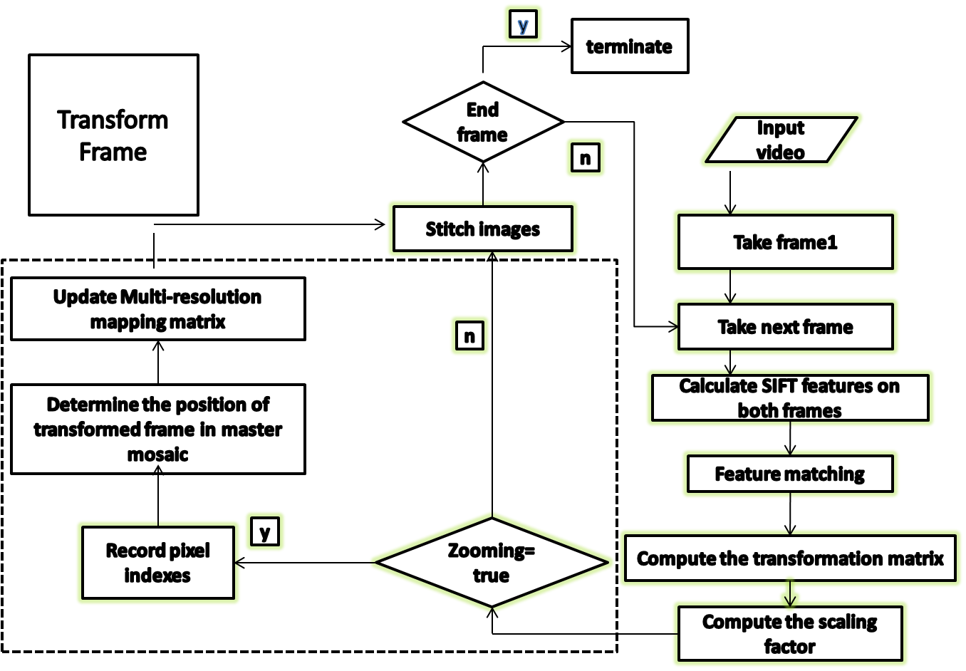 | Figure 1. System Flow Diagram |
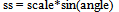
A. Feature DetectionFeature points are detected using Scale Invariant Feature Transform SIFT feature detector. Invariant scale features are also called SIFT features. SIFT features are local image features, which keep invariant in rotation, scale or illumination, and also robust in vision changes, affine changes or noises. SIFT algorithm is robust in detecting feature points. SIFT algorithm is also complex and inefficient. The time complexity of algorithm is high[1, 12].Following are the major stages of computation used to generate the set of SIFT features. See[9] for details.1. Scale-space extrema detection: The first stage of computation searches over all scales and image locations. It is implemented efficiently by using a difference-of- Gaussian function to identify potential interest points that are invariant to scale and orientation.2. Keypoint localization: At each candidate location, a detailed model is fit to determine location and scale. Keypoints are selected based on measures of their stability.3. Orientation assignment: One or more orientations are assigned to each keypoint location based on local image gradient directions. All future operations are performed on image data that has been transformed relative to the assigned orientation, scale, and location for each feature, thereby providing invariance to these transformations.4. Keypoint descriptor: The local image gradients are measured at the selected scale in the region around each keypoint. These are transformed into a representation that allows for significant levels of local shape distortion and change in illumination. Each keypoint is represented by a 128 element feature vector.B. CorrelationIt is required to find the correspondence between the SIFT features extracted. The indexes of the 2 sets of SIFT descriptors are determined that match according to a distance ratio. The distance between all pairs of descriptors in two corresponding sets of descriptors is computed. If ratio is smaller (or it is found to be in the threshold probabilistic way) to the given Distance Ratio, indexes will be zero for this entry. C. Determine the Scaling Factor After obtaining the points of correspondence between two successive frames, it is possible to generat correspondence maps between the two images. These correspondence maps can be used to combine the images into an aggregate structure.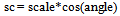 | (1) |
 | (2) |
 | (3) |
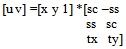
 | (4) |
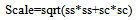
Here, sc specifies the scale factor along the x axis; ss specify the scale factor along the y axis. tx refers to translation along x-axis and ty translation along y-axis. In this way using matlab transformation function spatial transformation matrix is obtained. From the transformation matrix the scale is obtained. Linear conformal transformations can include a rotation, a scaling, and a translation. Shapes and angles are preserved. Parallel lines remain parallel. Straight lines remain straight. Based on the observations and experiments, the scale threshold is set to 0.9. If the scale factor is less than the threshold the current frame is zoomed with respect to the reference frame.D. Resizing Zoomed Frame and Preserving PixelIntensitiesThe high-resolution frames represent the regions in video sequence, where the camera zooms in, to capture any object of interest at higher resolution. For the zoomed frame the scaling factor is observed to be less than the specified threshold. The zoomed in frame is resized using bilinear interpolation so that it could align with the reference image. Consider following sequence of successive frames in Fig 2, where every next frame is at higher resolution than the previous one. 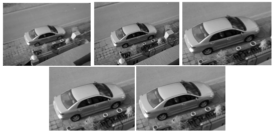 | Figure 2. Sequence of Zoomed Frames |
As shown in Fig 2, when the camera zooms in, resolution of the vehicle is increased step by step in successive frames. Due to resizing of zoomed frame for allignment, number of pixels in the interpolated frame is reduced, resulting in information loss. The aim of the proposed technique is to preserve the information lost in resizing.For bilinear interpolation, the output pixel value is a weighted average of pixels in the nearest 2-by-2 neighborhood. Loss of original pixel intensities during interpolation is demonstrated in Fig 3. In the proposed technique, for each pixel P in transformed image the x and y indexes of P (1, 1) are saved. Thus from the initial index the indexes of rest three neighbouring pixel indexes can be computed. | Figure 3. Bilinear Interpolation |
The scale would determine the size of the transformed image. Let I be the zoomed image and It be the transformed image after interpolation. Let r1 and c1 be the rows and columns in the zoomed frame initially than after resizing: | (5) |
 | (6) |
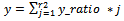
here r2 and c2 are rows and columns of the transformed image It. The row and column ratio of zoomed image I and transformed image It is calculated as follows: | (7) |
 | (8) |
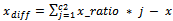
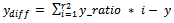
x_ratio and y_ratio is used to calculate the x and y coordinates of the pixels in the zoomed image I which are contributing in the computation of interpolated pixel intensities in transformed image It. The x and y coordinates of the pixels in the zoomed image I are calculated as: 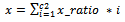 | (9) |
 | (10) |
 | (11) |
 | (12) |
Where  and
and  are the x and y coordinates of the pixels in the zoomed image I. As described earlier that if the initial indexes for any pixel ‘P’ i.e.,
  and
and  are stored, for each pixel in the transformed image, the actual pixel intensities can be retrieved from zoomed frame.The total number of pixels in the resized image would be r2*c2. Therefore it is required to record r2*c2 indexes in order to create a mapping matrix from mosaic image to the real zoomed in intensities for each pixel in the image matrix. Thus it is required to create a data structure of the same size as the mosaic image that would keep track of the pixels having zooming information and pixels without zooming details.
 | (13) |
 | (14) |
 | (15) |
 | (16) |
 | (17) |
 | (18) |
Where A, B, C and D are the four closest pixel values which are used in bilinear interpolation as follows and then assign a single value to the output pixel by computing a weighted average of these pixels in the vicinity of the point. The weightings are based on the distance each pixel is from the point.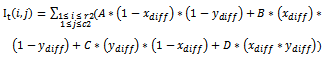 | (19) |
Where  refers to the interpolated image pixel intensities in the transformed image. Our proposed technique makes use of saving indexes rather than the pixel intensities A, B, C and D, which compose the interpolated image intensities. Fig 4 shows the interpolated resized image and corresponding zoomed frame .Here it can be seen that A, B, C and D are the four closest pixels. Now the four actual intensities are lost and a new single intensity value is formed. Therefore it is needed to keep track of the composing four pixel intensities for each pixel. There are two ways this idea can be implemented; either by recording the indexes of the composing pixels or by recording the pixel intensities . The first approach is preferable. The idea is efficient in terms of time and memory requirements, as it is needed to record only x and y index of one initial pixel, instead of saving four intensity values for each pixel in interpolated image. Besides this lot of redundant information would be stored e.g. if pixel 1 is formed from pixels (2,1),(2,2),(3,1) and (3,2) and pixel 2 is formed from(3,1),(3,2),(4,1) and (4,2) than redundant information is saved if four intensities for each pixel are stored. For high resolution images, this would consume lot of memory.Hence, it is required to record x and y coordinates of ‘A’ i.e.,
  and
and  for each interpolated pixel in It. If the size of the transformed image It is r2*c2, it is required to have a data structure that stores r2*c2 ‘x’ and ‘y’ coordinates. E. Formation of Multi-Resolution Mapping MatrixSince during image transformation, many pixel intensities are lost and the details in zoomed image are no more visible in the final mosaic image . In order to record the initial indexes of composite pixels, a multi-resolution data structure is proposed that creates efficient mapping from mosaic to the original zoomed pixel intensities.For example consider a 240*320 mosaic image. In Fig 5, a data structure is shown whose size is equal to size of mosaic image which shows how maximum zoom intensities, for each pixel in a 240*320 mosaic image are stored. ‘0’ against any pixel represents that this pixel do not contains any zooming information. Whereas the non-zero values for any pixel represent the indexes of first closest pixel contributing towards formation of its interpolated intensity.Whenever an image is zoomed, some pixels are zoomed in whereas some pixels are not. Multi-resolution “mapping matrix” is used to keep track of zoomed and unzoomed pixels in the mosaic. For zoomed pixels, it keeps the starting index of the actual corresponding pixels in the original zoomed frame .As shown in Fig 5 the index x and y of pixel ‘A’ is only stored in the multi-resolution matrix. This index represents the first closest pixel in the actual zoomed frame. The indexes of rest three composing pixels B, C and D can be obtained from coordinates of A. In the following Fig 6, the indexes (2,1),(2,2),(3,1) and (3,2) are the four neighbouring indexes of A,B,C and D intensity values in maximum zoomed frame that have formed pixel 2 . As shown in Fig 6, corresponding to each zoomed pixel in mosaic image, there are four indexes represented. From theses four indexes the starting index i.e. (2, 1) for pixel 1 is stored in the map as shown in multi-resolution mapping matrix. These indexes correspond to the four neighbouring pixel intensities in the actual zoomed frame. Viewing The Region Of Interest Selected By The UserWhen the final mosaic has been created the user can scroll the mouse over the image and select a rectangular region of his interest. If the area selected by user, has any further resolution, it will be displayed.
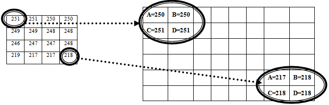 | Figure 4. Pixel Intensities Formation in Transformed Frame from Zoomed Frame |
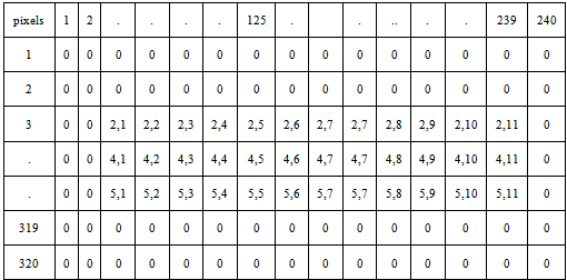 | Figure 5. Multi-Resolution Mapping Matrix |
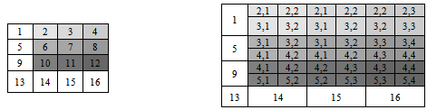 | Figure 6. Mosaic Image and Corresponding Zooming Indexes |
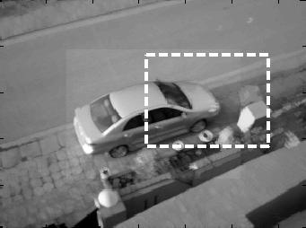 | Figure 7. Region Selected by User |
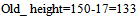
Fig 7 shows the region selected by the user. When the user selects the rectangular area, the starting and ending x, y coordinates of the area selected are saved, as shown by the circular marks in Fig 7. Three different cases can happen. First, the region selected contains some pixels that have zooming information and some pixels do not have. Second, none of the pixels in region have zooming information. Third, all the pixels in selected area have zooming information. Considering the first and the most complex case the rest two cases are also demonstrated. In the first case, it is required to create a “multi-resolution view” for the viewer. First, the pixels between the starting and ending points, marked in Fig 7, are traced in the multi-resolution “mapping matrix”. Those pixels that have non-zero indexes in the matrix have zooming information. As it is evidently shown in Fig 8, from the region selected, some pixels are zoomed, whereas some pixels are not. For example for the region selected in the mosaic in Fig 7, the starting pixel coordinates are (2, 10) and ending pixel coordinates are (220,133).As shown in Fig 8, the sub region containing zooming information and the sub region without any zooming information are indicated. It can be seen that pixels having zooming information, are starting from (x1, y1) i.e., (17, 20) and ending at (x2, y2) i.e. (150,133) in Fig 8. The size of the region having zooming information would be determined as: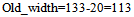 | (20) |
 | (21) |
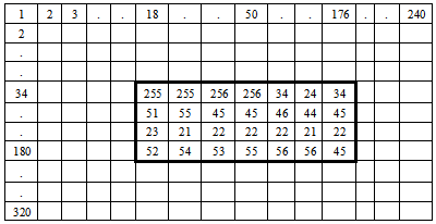
From Fig 8, it can be seen that, corresponding to the first zoomed pixel of region selected (17, 20), the coordinates are (34, 18) in the multi-resolution mapping matrix. Similarly for the last zoomed pixel of region selected (150, 133), (180,176) are the corresponding coordinates in the mapping matrix. These are the respective pixel indexes in the maximum zoomed frame. Therefore, the actual zooming details that are of viewer’s interest, are the pixel intensities that lie between (34, 18) and (180, 176) in the maximum zoomed frame, as shown in Fig 9.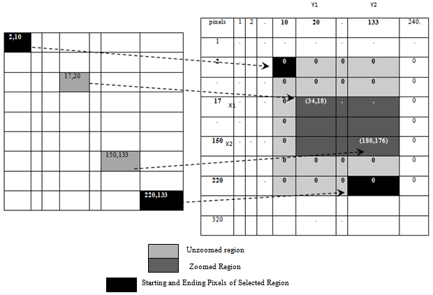 | Figure 8. Correspondence between Region Selected and Multi-Resolution Mapping Matrix |
 | Figure 9. Zoomed Pixel Information of Region Selected |
The width and height of the sub region having zooming information shown in Fig 8 would increase due to increase in number of pixels. The new width and height as shown in Fig 9 would be: 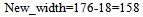 | (22) |
 | (23) |
Thus the “zooming factors” would be determined as follows: | (24) |
 | (25) |
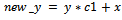
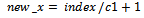
Zooming_x and Zooming_y are the scaling or zooming factors along x and y directions of the region having zooming information. Since there is some region in the area selected without any zooming information thus it is required to create a “multi-resolution view” user where the region with actual zooming information and the region having no zooming information are distinguishable. Let ‘rows’ and ‘cols’ be the rows and columns of the whole region selected by the user. The region with zooming information has greater number of rows and columns as compared to the region without zooming information. This is the hinderance in formation of a rectangular matrix that can be displayed using matlab display functions. To overcome this limitation, the region without zooming information is resized using the same scale or zooming factor. Therefore, the whole selected region would be first resized to new dimensions calculated as follows: | (26) |
 | (27) |
The resized image is shown in Fig 10. So the whole selected region is resized to New_rows and New_columns. In the resized image shown in Fig 10, some region has actually zoomed pixel intensities. The actual pixel intensities retrieved using the multi-resolution mapping data structure as shown in Fig 9 would merge in the resized image shown in Fig 10. It can be seen from Fig 8 that the pixels having zooming information, are starting from (x1, y1) and ending at (x2, y2) in the selected region. Therefore, it would be required to calculate the corresponding positions of starting and ending positions of the actual zooming pixel intensities block in the resized image. | (28) |
 | (29) |
 | (30) |
 | (31) |
For example (17, 20) and (150, 133) are the starting and ending x and y coordinates of the sub region shown in Fig 8, which are multiplied with the scale or zooming factors to get the exact positions of zoomed intensities block in image shown in Fig 10.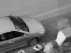 | Figure 10. Resized Whole Selected Region |
After placement of the original zooming intensities in the respective region in image shown in Fig 10, the final view for the user is obtained, shown in Fig 11 (b). It clearly shows the region having actual zooming intensities and the area without actual pixel intensities.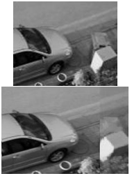 | Figure 11. Zooming Details of Region Selected (a) Region Selected (b) Zooming Information of Area Selected |
When the all the pixels in the region selected by the user have zooming detail it is simpler as compared to above mentioned case. The zooming intensities would be obtained as described in the previous case and displayed to the viewer.No merging of zoomed and unzoomed pixels is required. Considering the third case, where none of the pixels in the selected region have zooming information. Since, no information exists in multi-resolution mapping matrix for such pixels, as depicted by ‘0’ in the matrix. Thus the region would be simply resized by a factor of 1.25 and displayed to the user. That will make the user understand that there is not actual zooming information in the selected area. Image StitchingIn order to create the mosaic image it is needed to align the transformed image with the reference image. These images are placed on identical sized canvases and then combined to create the final image. Using the offsets of the transformed image with respect to the original image the images are aligned. The offset is calculated by using affine transformationThe offset of initial point of the transformed image with respect to the initial point of the static image can be positive or negative. This information along with the image sizes allowed for not only the summation of the transformed and static images, but also creates an appropriate canvas for the resultant image.
3. Results and Analysis
To prove the proposed technique, algorithm is tested on various video sequences. For carrying out analysis of proposed technique some parameters are defined. The qualitative parameters involve computational complexity, performance loss, processing overhead.The videos selected for experimentation are those which includes single object zooming. Since the proposed algorithm is a new algorithm and no such multi-resolution mosaicing algorithm exists so there is no comparative study performed with any other technique. A. Computational AnalysisTo prove our proposed technique, algorithm is tested on various video sequences. Execution time for various video sequences is shown in TABLE I. The results presented in TABLE I revealed that the algorithm is efficient. Execution time comparison is not given because no such multi-resolution mosaicing technique presented until now.| Table 1. Execution Time of Sequences |
| | Video Sequence | Number of frames | Total execution Time | | 1 | 45 | 51.03 seconds | | 2 | 67 | 98.5 seconds | | 3 | 85 | 103.6 seconds | | 4 | 85 | 86.99 seconds | | 5 | 42 | 33.13 seconds |
|
|
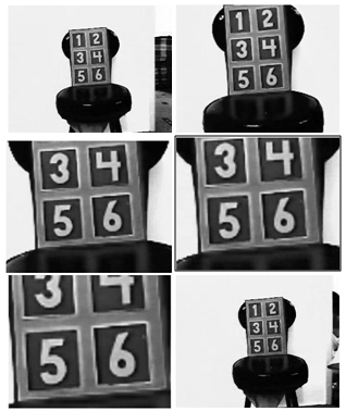
The technique is time efficient .Inspiteof the complexity and the huge computations involved in it,its execution time is good enough. As compared to simple mosaicing techniques, memory requirements of multi-resolution technique presented are high. The execution time is recorded by its execution in Matlab , by its implementation in other appropriate tools like C sharp, more efficient results are expected.B. Visual ResultsVisual results of mosaic are most important. Visual result of panorama depends on type of camera, environment and weather. Panorama created from video sequence 1 is shown in Fig 12. It was taken from digital handheld camera and noticeable intensity variation. Other two video sequences are taken from Sony digital camcorder with automatic camera control on brightness which causes intensity variation.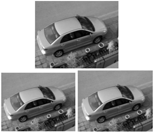 | Figure 12. Sequence of Video Frame |
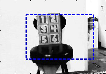
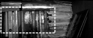
The algorithm correlated and created panorama successfully for all tested videos without any good guess for initial parameter. The first video includes a single zoom in motion. The complete scene of video sequence 1 is shown in Fig 13. 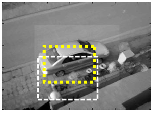 | Figure 13. Region selected in mosaic image |
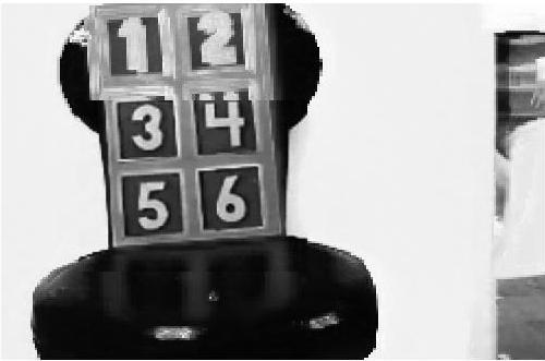
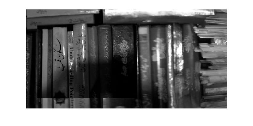
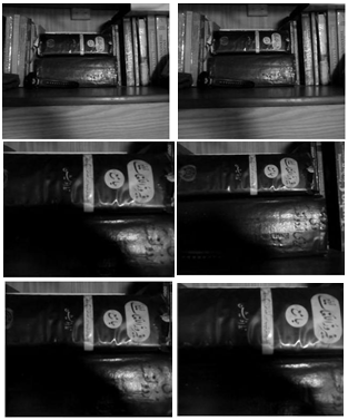
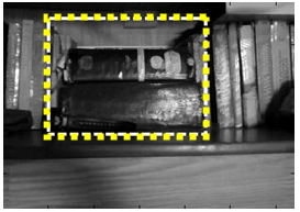
Fig 14 shows zooming information of the region selected from the mosaic image in Fig 13. The zooming details show that some pixels in the region selected have actual zooming information corresponds to the area in Fig 14 that is more clear. Fig 15 shows sequence of frames that includes a small pan and than zooming in and out motion ,followed by a small pan motion in the end. Fig 16 displays the mosaic and the region selected in it.Fig 17 shows the zooming information of the region selected .Fig 18 shows another video sequence that includes pan motion followed by a zoom motion..Fig 19 shows the mosaic and the region selected by the user.In Fig 20 the zooming information of the selected region is displayed.Fig 21 shows the frames of a video which includes single zoom in motion.Fig 22 displays the mosaic constructed and in Fig 23 the maximum zooming details of selected region are displayed.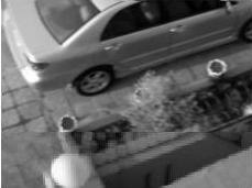 | Figure 14. Zooming Information of Region Selected |
 | Figure 15. Sequence of Video Frames |
 | Figure 16. Region Selected in Mosaic Image |
 | Figure 17. Zooming Information of the Region Selected |
 | Figure 19. Region Selected in Mosaic |
 | Figure 20. Zooming Information of Region Selected |
 | Figure 21. Sequences of Video Frames |
 | Figure 22. Region Selected in Mosaic |
 | Figure 23. Zooming Information of Region Selected |
References
| [1] | F. SONG, B. LU, “An Automated Video Image Mosaic Algorithm Based On SIFT Feature Matching,” American Journal of Engineering and Technology Research, 2011, Vol.11.No 9,2011 |
| [2] | Heikkila, M., Pietikainen, M., “An image mosaicing module for wide-area surveillance” In: Proceedings of the Third ACM International Workshop on Video Surveillance & Sensor Networks,Singapore, pp. 11–18 ,2005. |
| [3] | M. Irani, P. Anandan, J. Bergen, R. Kumar, and S. Hsu, “Mosaic Representations of Video Sequences and Their Applications”, Signal Processing: Image Communication, Special Issue on Image and Video Semantics: Processing, Analysis, and Applications, Vol.8, No.4, 1996. |
| [4] | H. Y. Huang and T. C. Wei, “Fast locating detection of covering region in image mosaic,” in Proc. of the 2nd European Workshop on the Integration of Knowledge, Semantic and Digital Media Technologies (EWIMT2005), pp. 301-308, IEE Savoy Place, London, UK, Nov.30~Dec. 1, 2005. |
| [5] | A. Bevilacqua and P. Azzari, “ A fast and reliable image mosaicing technique with application to wide area motion detection”,Proc. of ICIAR 2007 , pages 501-512, August 2007. |
| [6] | Zhi Qi and J.R. Cooperstock. “ Depth-based image mosaicing for both static and dynamic scenes”. International Conference on Pattern Recognition, 1-4, 2008. |
| [7] | Su, M.S., W.L. Hwang, and K.Y. Cheng. “Analysis on multiresolution mosaic images”, IEEE Transactions on Image Processing, 13(7):952–959,2004. |
| [8] | Li, J.S., Randhawa, S.: “Improved video mosaic construction by selecting a suitable subset of video images”. In: CRPIT ’04: Proceedings of the 27th conference on Australasian computer science, Darlinghurst, Australia, Australian Computer Society, Inc. 143–149, 2004 |
| [9] | L.A Teodosio and W.Bender,”Salient Video Stills:Content and Context Preserved,”ACM Int,l Conf.Multimedia,ACM,NEWYORK,1993. |
| [10] | I. Trotts, S. Mikula and E. G. Jones, "Interactive visualization of multiresolution image stacks in 3D," Neuroimage 35(3), 1038-1043 ,2007. |
| [11] | R. Szeliski and S. Kang. “ Direct Methods for Visual Scene Reconstruction”. In IEEE Workshop on Representations of Visual Scenes, pages 26–33, Cambridge, MA, 1995. |
| [12] | Li, Y., Wang, Y., Huang, W., Zhang, Z.: “Automatic image stitching using sift”. Audio, Language and Image Processing, 2008. ICALIP 2008. International Conference on ,568–571, July 2008. |
 Abstract
 Reference
 Full-Text PDF
 Full-Text HTML