1. Introduction

New uses for aerial imagery as both reference and medium spur an ever-increasing need for tools to quickly and cost-effectively mosaic this imagery for scientific analysis. Such data sets are typically structured and complex, often including Uniform Transverse Mercator (UTM) coordinates, digital elevation data, and several other parameters like roll, pitch and heading telemetry along with visual and LIDAR (Light Detection And Ranging) or infrared information. The near future holds innumerable imagined uses for such systems, because new forms of analysis that use these data sets are being imagined and realised daily. The need for automatic systems to perform, check for errors in and correct aerial image registration is great, in terms of both reducing tedium for and exceeding the capabilities of a human operator.

Collecting aerial imagery is conceptually straightforward. The aircraft flies back and forth overhead while the on-board sensor platform records a wealth of data about the terrain below. A visible spectrum camera captures images at a 10° forward angle, to align with LIDAR, at regular intervals, creating a sequential set of overlapping images, arranged in lines. One group of consecutive lines is captured during the first half of the flight, and another set of lines is overflown between the outgoing lines, on the way back to the airfield.

Associated with each image is a host of data, contained in a DAT file. Data associated with each line of this file includes path and file name, northing and easting values, elevation in meters, roll, pitch and heading values in degrees, and UTM grid number. The remainder of the data contained in this line is superfluous for our purposes. The Mosaic program uses the noted information to place each image center on the UTM grid.

The Mosaic program aligns several hundred to a few thousand images to provide a better means of analysing the data they represent. When applied to only two images, this is the basic definition of image registration. The sensed image is moved into alignment via some means of assessing the match, usually the reference image. In this case, each image is placed on the UTM grid based on its projected location relative to the aircraft's position and attitude.

To find the UTM coordinates of each image center, Mosaic projects the vector normal to the camera lens onto the UTM grid using the aircraft roll, pitch, heading and altitude associated with the image in the DAT file combined with the Digital Elevation Modelling (DEM) file terrain elevation[1]. Because the images overlap, the appropriate pixels to include from each file are selected by a Voronoi diagram. The diagram associates the optimal pixels, those closest to the image center, with the center of their originating image and therefore the appropriate image number to use for the actual, pixel by pixel mapping of the mosaic.

2. The Bore Sight Estimator

The process of calibrating the relative roll, pitch and yaw of the camera with respect to the airplane is referred to as bore sight estimation. This is necessary when the sensor platform is removed and replaced or occasionally due to vibration and shock. The BSE program analyses a relatively small group of images to augment the Mosaic program's accuracy, providing a single, vector adjustment to the attitude parameters of every image in the data set[1].

To assess alignment between images, the program creates chip pairs, rectangular subsets of the image space that are extracted from the same UTM coordinate defined regions of both the reference image and the sensed image. Chips are compared for matching content to determine alignment, and may range in size from 8 pixels by 8 pixels to the majority of the entire overlap area. Every chip pair is passed to a Hooke and Jeeves algorithm for evaluation. The algorithm finds a local maximum for Pearson's correlation, given a chip pair, as assessed at different attitude parameter values. Once their collective alignment is determined to be at an optimum, the resultant adjustment in the attitude vector will improve the alignment of the images when they are processed through the Mosaic program.

Chip pairs are generated along the Voronoi boundary, nearly equidistant to the image centers, at regular intervals on this border line. BSE sends all of these chip pairs to the Hooke and Jeeves algorithm, which will compute their adjustments separately as detailed below and average the result. The process is detailed here:

1. Start with the initial attitude vector, initial step size, step size reduction factor, minimum step size and maximum iterations.

2. For each chip pair, the chip from the neighbouring registered image is left static while the roll, pitch or heading of the chip from the sensed image is adjusted, one at a time according to the current parameters given by Hooke. Correlation is assessed.

3. Correlation return for every chip pair is averaged and, based on achieved improvement in this overall average, a search direction is determined and pursued on the next iteration. If no adjustment yields an improvement of correlative value, then the step size is reduced and the process is repeated.

4. At each step the values are retained for each parameter. The best search vector is thus retained.

5. Steps 2, 3, and 4 are repeated until either the step size is reduced below the minimum allowed or the maximum number of iterations is reached. In the first case, a local maximum correlative value is reached. In the second case, the program exceeds the maximum number of steps allowed, holds the best correlative value available within a finite number of steps, and has returned the best suggestion for image movement it could reach[1].

Once all chip pairs in the test data set have been put through this algorithm, the attitude parameters that locally optimise average correlation for all chip pairs is returned. This suggested adjustment is the purpose of the BSE program, and relates to the orientation of the camera. Once these values are adjusted by the offsets suggested by BSE, the Mosaic program can be run again, providing a better mosaic.

3. Finding Problem Images

The Mosaic program turns a time-wise flow of images into a position sequence of images via a projected vector as a transformation function that is capable of mapping the overlapping pixels of one image into an almost exact match of the overlapped region of each its neighbours When an image and its neighbours are properly registered to the UTM grid, each will align well with the others. The system accounts for flight attitude parameters and image perspective by adjusting the coordinates of the image center away from the aircraft location coordinates as recorded in flight telemetry. This system does not address inaccuracy of flight attitude parameters as reported in aircraft telemetry. Since these parameters are used in computing the placement of the images, if they are reported inaccurately the transformation will be inaccurate.

Several sources mention the inherent instability of small aircraft as a platform for aerial sensors as inducing error in registering images or in accurately locating a particular image on a GIS or other location-based grid[3-5],[7],[11]. During normal flight, the aircraft maintains a sufficiently stable attitude for the projection scheme described above to place the image center within no more than one to two pixels, and often within one half pixel, of precise alignment. When the aircraft incurs excessive crosswind, thermal currents, wind shear, or other turbulence, the sensors may not record accurate values for one or more of the flight attitude parameters. Whether under or over reported, the result is the same. Aircraft position closely follows the center of mass of the aircraft, which describes a roughly straight line. The vector projected, based on the improperly reported parameters, references the wrong location on the UTM grid. The result is that the image center will be placed improperly by the Mosaic program.

Since the pixels of an image file are mapped directly through the transformation function to the UTM grid according to the vector projection plus an offset from image center, every pixel of the constituent image will be improperly placed. Visually, this is only detectable along the Voronoi diagram boundaries, where the pixels of the improperly placed image meet the pixels of its presumably well placed neighbours, creating a misalignment. These discontinuities are observable as sidewalks, streets, roof lines, or other normally continuous features that do not match up across boundary lines.

The Alpena, Michigan data set evaluated for this investigation contains 1,249 images. The majority of these images have an associated parameter set that projects the image center to within one or two pixels of precise placement. Roughly 12% of the images from this set, though, exhibit a characteristic that places them outside of this envelope and approximately 5% of the set will benefit from mitigation. The proposed process automatically detects these images. Once found, their parameters can be adjusted similarly to the process described for the BSE program above, providing a new, more accurate transformation function vector, but for the individual image instead of the whole.

When graphing the image centers in an attempt to find deviations from the linear nature of flight lines it was observed that the aircraft center coordinates for each image form nearly straight lines when graphed as easting values (x axis) versus northing values (y axis). The image centers, as adjusted by the Mosaic program, were comparatively erratic. The latter should have been fairly linear, given negligible environmental conditions. The next step was to graph the image centers as reported by Mosaic, then compare each flight line to a linear regression of itself as shown in figure 1, which features a specific area of the flight line containing image 446.

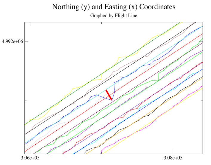Figure 1. Some image coordinates show greater deviation from the flight lines than others, like image 446

Note the thick, red line in figure 1. It represents an indicator of the error this image will exhibit. Since its center is so far from the linear approximation, one or more flight attitude parameters must be causing the projection to produce this deviation, as these are the parameters Mosaic uses to place the image. This indicator will be calculated as a Pythagorean product and can be treated as an RMS error because we have found that some combinations of roll, pitch and heading, that do not deviate significantly on their own, combine to produce visually identifiable mosaic errors that are identifiable by this process. To find the coordinate deviation associated with each image, northing and easting coordinate data from each flight line were imported into XMGrace and a linear regression was performed on each set. The linear data sets were then exported back into the original ASCII file alongside the corresponding Mosaic northing and easting data. An Awk script then took the differences and computed the Pythagorean distance from the linear approximation to the actual value. Once the file was sorted in descending order, based on the error column, the top of the file became a list of problem images like image 446 shown above.

While this process was a good beginning, it did not accurately predict every misaligned image found during visual inspection. Images like 446 made the list, due to the extremity of their misalignment, but more subtle discontinuities were still found ranked beneath seemingly well placed images. Additionally, cases of excess yaw, rotating the image but not seriously displacing its center, were not detected by this process.

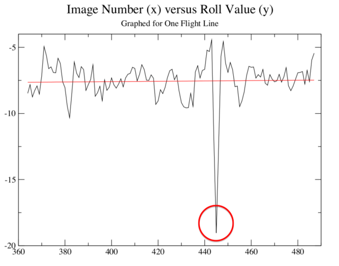Figure 2. Roll values for the flight line containing image 446

To address the source of the coordinate based error, each flight attitude parameter was analysed just as easting and northing were, but no Pythagorean step was necessary as these parameters are one dimensional. Each was imported into XMGrace, where a linear regression of each flight line was performed. The linear data was exported back to the original file where the difference between actual and estimated values were calculated and the absolute values taken. The result was three files, one each for roll, pitch, and heading, that were sorted in descending order on the magnitude of the observed error. These three files were excellent predictors of the images found via visual inspection, and led to the discovery of several, more subtle errors not detected during visual inspection. An example of this error is shown in figure 2. Note that our case image, number 446, deviates significantly from the linear estimate. While roll was the most obvious indicator, graphically speaking, pitch and heading values exhibited similar characteristics.

As a further refinement, a composite error was computed as the square root of the sum of the squares of the roll, pitch, heading, and location based errors. This was also done via Awk script, and the sorted results highlighted a few more images whose subtle errors had combined to make the overall misalignment of each greater than that of the images considered to be normal. The final step in detecting the problem images was to select a cutoff point, below which errors would not be considered significant. Visual inspection revealed that a cutoff of roughly one standard deviation above the mean error was found to be fairly inclusive without encompassing too many well placed images. This turned out to be approximately 40 images from the top of each file, amounting to roughly 200 images. After the redundant images were removed, 148 unique images were suggested by the process as likely to generate mosaic errors. These images were processed using the Hooke and Jeeves algorithm described below. Their attitude parameters were adjusted and the mosaic was remade using the new values for these images.

4. Correcting Parameters via Hooke and Jeeves

Each image from the data set will have several neighbours Assuming that these are registered properly on the UTM grid, bringing the wayward image into alignment with its neighbours will also register it accurately against the UTM grid. This process will also mitigate any discontinuities observed at the borders. The process is much like that detailed above for the Bore Sight Estimator, except that the known features used as reference are the chip pairs of neighbouring images not identified by the process. Provided that the chips from the neighbouring images are well placed on the grid, they can serve as reference points.

Unlike BSE, only one sensed image at a time was processed. Every neighbour was used, generating chip pairs in the overlapping area common to the image pair, until it has created on the order of 30 to 150 chip pairs, depending on the chip size selected.

Chip pairs were generated along the Voronoi border, then that line was rotated 45°, 90°, and 135°, generating a new group along each of these lines, flooding the overlap area with chip pairs. It was observed that, when the chip census was low or the Voronoi boundary exists in a low pixel intensity variance area, the average of the chips' suggested adjustments was skewed due to a greater standard deviation of these values. Besides a greater number of chips with more varied locations, a variance filter was applied. No chip pair was reported as viable unless the pixel intensity variance of both of its constituents was above a floor value; 0.2 was the value that returned the best results.

Armed with more chip pairs, covering more of the overlap area, and with the variance filter, the poorly registered images were processed, one at a time, through the Hooke and Jeeves algorithm as it is explained above for BSE. The algorithm used every chip pair created and validated, averaging the return from a correlation function coded specifically for the purpose and discussed below, to guide the algorithm to returning an adjustment specifically tailored to the image in question. The output roll, pitch and heading values were then written directly to the appropriate line in the DAT file. Once each image had been processed and its new vector recorded, the Mosaic program was rerun on the data set and the resultant mosaic was visually compared in QGIS to the uncorrected mosaic.

Pearson's Correlation, or the covariance of the two samples divided by the product of their standard deviations, was used to assess the correlation, or alignment status, of a pair of chips created from two overlapping images. Pearson's correlation function provides a number between 0 and 1.0, inclusive, with 1.0 being a perfect match. When expressed slightly differently from the usual, computing means is unnecessary and the statistic can be coded to be computed in one pass. Since it was coded specifically for this application, its code remained local, providing an added advantage in efficiency. This was important as the Hooke and Jeeves algorithm calls it for every iterative evaluation of every parameter. As called, the function receives the image number and associated roll, pitch, and heading values suggested by the current iteration of Hooke. Each image has a list of chip pairs associated with it and its neighbours The function sums pixel intensity values, squares, and products for the entire area of both chips as read in from their respective arrays. The correlation is then computed and checked for a nonzero denominator, and the correlation value is reported back to Hooke so the algorithm can make its determination as to how to adjust the single parameter currently under consideration.

5. Image 446, a Case Study

Image 446 has served as our worst case. From the beginning, it was identified first visually due to the obvious nature and the magnitude of its misalignment, then by the suggested movement of its chip pairs, and finally by our process, due to its roll, pitch, yaw, UTM and combined scores. Every border of this image, displayed as figure 3, has fairly clear edges that exhibit obvious discontinuities. It was not only the most obvious, but the best test case as well because any improvement due to any mitigating method could be judged summarily, with the naked eye.

Considering the post-adjustment example, figure 4, makes this point clear. The edges in question line up almost exactly. Alignment of this image has improved dramatically within the mosaic. All three flight attitude parameters were adjusted quite severely when compared to the rest of the images from the data set. Although it took an entire afternoon of manual adjustment to this particular line in the DAT file, the test program accomplished this adjustment of parameters in less than five minutes.

Figure 4 demonstrates visually how precisely the alignment of the image was adjusted. Note how close the lines in the parking lot are to perfect alignment. While it is possible to look at the misaligned features in figure 3 and judge some of them to be as much as 5 m apart, it would be difficult to detect misalignment of the same lines in figure 4. Both versions of the mosaic were opened in QGIS for comparison. A distinct feature was visually selected at UTM coordinates 307102.0 easting, 49910040.7 northing. This feature was translated to 307097.7 easting, 4991034.3 northing by the roll, pitch and heading adjustments via Mosaic, for a difference of 4.3 m easting and 6.4 m northing. The corresponding Pythagorean distance translated for image 446 is approximately 7.7 m. Since this image was the test case and the worst in terms of visual and real misalignment with the surrounding mosaic, it represents the largest movement made by the process. Corrections to most other images ranged from one to two meters, but were nonetheless obvious improvements.

Table 1. Adjustments Made to Image 446 Parameter Initial value Final Value Adjustment Roll -12.40532 -12.55344 0.14812 Pitch 8.28528 8.37484 0.08596 Heading 123.50002 123.81445 0.31443

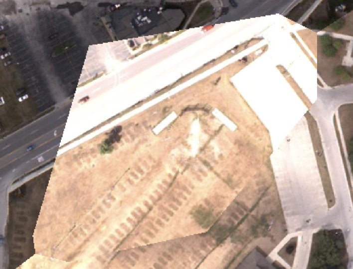Figure 3. Image 446 exhibits discontinuities as mosaiced before detection and attitude parameter correction

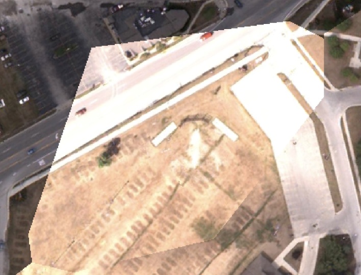Figure 4. Image 446 as mosaiced after flight attitude parameter adjustment

6. Conclusions

The combined list was compiled for the Alpena, Michigan data set. The process selected 148 images, almost 12% of the total of 1,249 images, for preprocessing. Of these, several were over water and several more were not in need of mitigation. The remaining approximately 5% of the image set represented good candidates for individual preprocessing. The most extreme errors displayed misalignments of as much as 4 to 5 m, or approximately 10 to 12 pixels. Most errors, though, were significantly lower in magnitude. Figures 3 and 4, and the QGIS analysis above, both demonstrate the effectiveness of this process in correcting alignment errors. The mitigation of these images validates the entire detection to correction cycle. While some images, such as our case image, showed up in more than one list, others were only reported by one parameter. Each parameter list was analysed and found to lack redundancy in reporting error. That is, each list contributed some unique image numbers to the master list and the master list would not have been comprehensive without the inclusion of all attitude parameters and UTM error, as well as the composite list.

Finally, as the correction of image 446 demonstrates, the Hooke and Jeeves algorithm combined with Pearson's correlation is effective at correcting flight attitude parameter errors. Other images from the list, while not such dramatic examples, also showed significant improvement across the board, exhibiting corrections of smaller degrees per parameter that translated to fewer meters of correction. Of further note, running the Hooke and Jeeves correction on correctly registered images had little or no effect, so exceeding the master list would do no harm to the mosaic.

7. Future Work

The correlation function used by Hooke is one area where improvement might be sought. Changing its composition might improve the necessary chip size, increasing the efficiency of the algorithm. Such changes might also make the correlation coefficient better for comparing the alignment of one image to that of another. Currently, achieving the best value attainable for one image and its neighbours works for aligning the image, but consistency of results across the spectrum of image composition, if attainable, will result in a uniform means of comparing the alignment of an image with its neighbours to that of another problem image and its neighbours, possibly even replacing the identification portion of the process.

Automation seems an obvious next step. The steps performed using Awk and XMGrace, outlined above, detail a provable, repeatable method for identifying problem images. Now that this process has been mapped, programming it in C++ or a similar language would speed up the process greatly. The level of error chosen as breakpoint, level of variance for the chip filter, and Hooke and Jeeves entry and exit values could be added to the parameters file or input through the startup script. The preprocessor could analyse the DAT file attitude data while the images are being read, and the problem images could be processed in parallel, one image per node as nodes become available. Libraries are available for the linear regression of the flight line data as well as the Awk and sort manipulations. Such a scheme would add, perhaps, as little as five minutes to the front end of the Mosaic program's processing time. While this time is significant compared to the 20 seconds Mosaic takes on the 16 core machine it currently runs on, it is significantly less than the time to perform these tasks manually, the result is a much improved mosaic with little human intervention, and the preprocessor could be set up to be bypassed by the user.