Ekaterina M. Fedotova, Igor A. Brigadnov
Department of Computer Science, St. Petersburg State Mining University, St. Petersburg, 191186, Russian Federation
Correspondence to: Ekaterina M. Fedotova, Department of Computer Science, St. Petersburg State Mining University, St. Petersburg, 191186, Russian Federation.
| Email: |  |
Copyright © 2012 Scientific & Academic Publishing. All Rights Reserved.
Abstract
The problem of minimization of ill-conditioned functions is considered. These functions are motivated by the limit analysis problem for dielectrics in powerful electric fields. From computing point of view a minimization of these functions is not following by standard methods because they are nonsmooth. Distinct ravine of objective function in combination with a high dimension variables requires a smooth regularisation of finite-dimensional problem. Convergence of heave-ball method in relation to it’s internal parameters and optimization parameters are studied in numerical computing environment and fourth-generation programming language Matlab.
Keywords:
Nonsmooth Functions, Smooth Regularization, Ill-Conditioned Problem, Numerical Minimization
1. Introduction
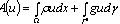
Investigation of electrical strength of dielectrics particular interest in both theory and practice[1]. It is stimulated by significance and practical interests in field of electrical engineering and microelectronics. When dielectrics are located in powerful electric fields it appears there the effect of loss of global electrostatic balance state between external electric field and dielectric. This effect we interpret as electrical puncture of dielectric[3-7].The electrical state of a medium in the given domain is characterized by the bulk  and surface g density of charges and by the vectors of electrical tensity E, electrical induction D and electric current density J. Vector D is introduced by the rule
 , where
  is the electrical constant, and P is the vector of polarization. For the electrical tensity the scalar potential u is introduced such as
 .In weak electrical fields the currents of conductivity in dielectric media are practically absent, i.e.
  , and the simplest linear constitutive relation
  is used[1]. As a result, for the solution of the appropriate linear BVPs, various effective analytical and numerical methods have been worked out.
2. The Limit Analysis Problem in Electrostatics
In powerful electrical fields the essentially nonlinear phenomena of polarization saturation  and ionization
  must be taken into account[1]. As a result, the integral model of bounded electrical induction is used, where
  and
and  is the complementary physical parameter of dielectric medium (the parameter of saturation) which is easily calculated[3-7].From the physical point of view this effect is interpreted as loss of the global electrostatic balance state between external electric field and dielectric on the analogy of loss of the load-carrying capability of solids in mechanics[7].Let a dielectric medium occupy a domain
 . It’s described by two vector-functions
 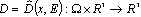 and
and 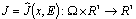 .We consider the following boundary-value problem. The quasi-static electrical influences acting on the dielectric are: a bulk charge with density
  in
in  , a surface charge with density g on a portion
  of the boundary, and a potential
  on a portion
  of the boundary is also given. Here
 ,
,  and area(Г1)>0. Point charges absent.We assume that from the classical Thomson's principle[1] it follows that the free energy of the electrical field in dielectric has the global minimum on the real potential, i.e. the potential u is the solution of the following variational problem:
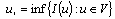 | (1) |
where: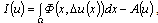 ,
,  ,where
 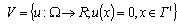 is the set of admissible electrical potentials, A(u) is the work of the electrical field on the external charges, Ф is the specific full energy of the electrical field such that
  for every
  and almost every
 . In the general case, according to the Thomson law and Joule-Lenz law specific potential energy of electric-field with regard to noninvertible losses from the current of conductivity is searched by formula:
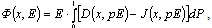 | (2) |
where point is the scalar product in R3.In the work[3] it is shown that there is always exists such parameter of electrostatic saturation λ>0, that for any  and almost all
  an estimation is faithful:
 | (3) |
A solution for the problem (1) can be absent. Physical sense of this effect is that a dielectric can perceive a limited amount of the electric fields that is interpreted as a loss of electrostatic equilibrium between externals source of electric field and dielectric. This effect we call as electrical puncture of dielectric.In the work[3] it’s shown, that analysis of electrostatic equilibrium in a dielectrics is reduced in order to research parameter , such, that for
  functional
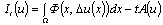 | (4) |
is limited on V and it’s proved, that for  an estimation above
  is correct , where
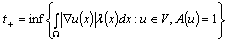 | (5) |
and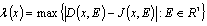 .Solution of the given problem is reduced in[3] to substit (4) by the solution of next problem:
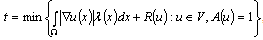 ,and more precisely to research of properties of function R(u), having next view:
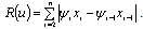 | (6) |
It is possible to show by a simple example, that without boundary conditions, i.e. without fixing actual value of first or last variable, an objective function (6) achieves at minimum on a linear variety. In other words, an objective function has an endless number of points of minimum. For example, function of three variables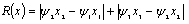 achieves at a minimum value
  for all variables fulfilling a condition:
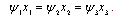 .Through the variational-difference method based on finite-element piecewise linear approximation of the required solution, an initial continual problem (5) is reduced to the next finite-dimensional problem of minimization of uneven function of kind:
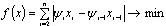 | (7) |
The function (7) is a convex function, but it is nonsmooth because it’s a sum of the modules, that does not allow to apply the standard methods of minimization, for example, gradient or Newton’s methods. Even more, the simplest coordinate descent minimization requires a continuously differentiable (smoothing) objective function for the convergence[8].For application of standard methods of minimization it is necessary to smooth out this function, i.e. to carry out it’s regularization.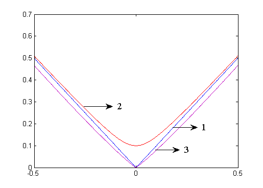 | Figure 1. Regularization of the module at a value ε=0,01 |
1 – is the initial function of modulus;2 –
 is the regularization above;3 –
 is the regularization near x=0.We suggest to use the third variant - regularization near x=0, since it’s more natural, saving basic properties of modulus function in the neighbourhood of singular point. As a result, a finite-dimensional problem takes the following form:
 , where
  is a small positive parameter (
 ). In this case the object function is ill-conditioned.Ill-conditioned functions are characterized by that slight changes of basic data can result in the massive changes of solutions. We remind that the condition number of a matrix A is
 ,possessing properties
  and
and  , where
  are eigenvalues of the matrix A.Matrix A is named ill-conditioned if
  . In practically important problems the condition number can evaluate too large as (106-109).Function
  is named ravine, if its hessian can be ill-conditioned matrix.The original objective function is attributed to the class of functions of ravine type, for minimization of which a number of the special methods has been worked out. We have chosen the heavy-ball method, since this method is master of the certain set of properties allowing effectively resolve problems of minimization of ill-conditioned functions[9].Heavy-ball two-step method is lookup method of global minimum and its modification of gradient method.Finding a solution of the problem with the help of gradient methods consists of some steps: beginning from some starting point
  are realized consequent steps to some other points unless acceptable solution of problem will be found.Gradient method for solution of problem of absolute minimization
 | (8) |
where f: Rm → R, it is possible to interpret in terms of usual differential equations in such a manner. We will consider next differential equation | (9) |
(here the above point x is the derivative on the independent variable t, and f ′(x) as usual means the gradient of mapping: Rm → R; it is assumed that p > 0). The simplest finite-difference analogue of equation (9) has the view of obvious chart of Euler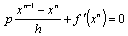 ,gradient method for problem (7) is written as
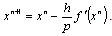 | (10) |
Consider now instead of equation (9) the following equation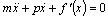 | (11) |
describing motion of the ball of mass m in the potential field f ′ in presence of friction force. The loss of energy on a friction will force a ball to get down pithily a minimum of potential of f, and forces of inertia will not allow to oscillate how it is represented on a chart. It allows to hope that change of equation (9) by introduction an inertial member will improve the convergence of gradient method (10). The finite-difference analogue of equation, describing motion of a ball: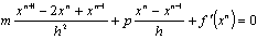 After simple transformations and obvious labelling we get a next iteration scheme:
 | (12) |
that describes the heavy-ball method to solve the problem of absolute optimization of ravine functions. 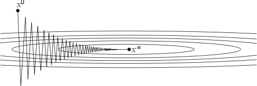 | Figure 2. Gradiend method |
 | Figure 3. Heavy-ball method |
3. Numerical Experiments
Numerical experiments were carried out in numerical computing environment and fourth-generation programming language Matlab. In the program was entered numerical vector of coefficients , parameter of regularization ε, parameters α and β for calculations according to the heavy-ball method and precision of calculations δ.
3.1. Program Development
The program in Matlab was carried out in the form of M-files. The modules were implemented by corresponding M-functions.The module of data control checked nonnegativeness of precision δ and parameter ε and was implemented in the body of M-function for calculations according to the heavy-ball method.Module solving problem according to the heavy-ball method was implemented as a separate M-function. For that function parameters α, β, ε and precision δ were fixed by user through the Command Window.The module for the calculation of gradient was implemented as a separate M-function called in the process of calculations in the module, solving the problem according on the heavy-ball method.
3.2. Testing of the Program
Before using the program, it was necessary to carry on testing with the aim of verification of all functions that the program must execute and verification of a response of the program in different situations.It was necessary to conduct next tests to define influence of different factors, such as:-precision δ;-parameter of regularization ε;-parameters α and β for the heavy-ball method.For the verification of the program the method of testing described above was used on the example of the problem a decision of that is easily determined analytically, or in the Matlab. With the aim of the comparison of the efficiency of different algorithms special test functions having essential singularities on extremum lookup are developed. One of well known is a Rosenbrock function, that was used for testing of the complex program.For testing the program vector of coefficients with dimensionality n random number generator was used.For estimation of influence of the precision on the quantity of iterations parameter ε and precision of calculations δ were changed with constant dimensionality of the vector of coefficients and parameters α and β.For estimation of the sensitivity of heavy-ball method to the parameters α and β with the constant dimensionality of the vector of coefficients, precision and parameter of regularization parameters α and β we changed itself in given diapason and quantity of iterations was measured.For estimation of influence of the parameter of regularization ε on the quantity of iteration with the constant dimensionality of the vector of coefficients, parameters α and β and precision δ was changed parameter of regularization itself in given diapason and quantity of iterations were measured.
3.3. Results of Numerical Experiments without Considering of Boundary Conditions
3.3.1. Dependence of the number of iterations on parameter of regularization ε
At the fixed value of precision δ=0.1 and β=0.1 there was a next picture:At α=0.12 the number of iterations was 1 at any value of ε.At values from α=0.15 to α=0.13 and и ε=0.1 number of iterations was 1, then at ε<0.1 a process loopsAt α>0.16 the process loops at all values ε.
3.3.2. Dependence of the number of iterations on precision δ
At ε=0.1, ε=0.01, ε=0.001, ε=0.0001 dependence is identical.At precision δ=0.1 the number of iterations was 1, at δ<0.1 the process loops.
3.3.3. Research of sensibility of heavy-ball method to parameters ( )
)
We see distinctly, that at ε=0.1 the number of iterations rises sharply and a process loops at α>0.15, while at ε<0.1 the number of iterations rises sharply already at α>0.12.
3.4. Results of Numerical Experiments with Considering of Boundary Conditions
The analysis of problem showed that objective function without boundary conditions has an endless great number of points of minimum, located in a ravine area that results in the formal cycling of algorithm. As a result, for providing of unicity of decision the boundary condition of х(1)=2 was used. We will notice that an initial variation problem in natural way contains boundary conditions on the required function.
3.4.1. Research of Sensibility of Heavy-Ball Method to Parameters ( )
)
General view of chart of dependence of number of iterations from parameters α and β at precision δ=0.1 and ε=0.01.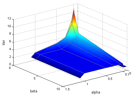 | Figure 4. Sensibility of heavy-ball method to parameters ( ) ) |
At different precision δ the peak of number of iterations is observed at different values α, that evidently from the brought 4th charts of dependence of number of iterations from the parameter α at the fixed parameters ε=0.01 and β=0.01.With the change of precision the characteristic peak of number of iterations evolves in the area of small values, in this process his size raises sharply.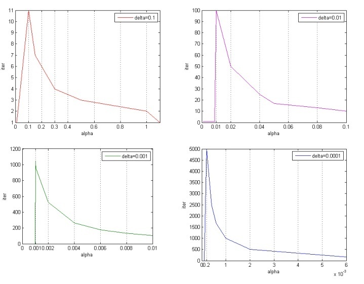 | Figure 5. Sensibility of heavy-ball method to parameters with δ=0.1, δ=0.01, δ=0.001 and δ=0.0001 |
3.4.2. Dependence of the Number of Iterations on Parameter of Precision Δ
The number of iterations was measured at the fixed values of parameters α=0.01 and β=0.01.From a chart is evident, that at precision δ=0.1 the number of iterations is small, at the increase of precision to δ=0.01 it increases sharply and then it changes insignificantly. Also it is obvious, that at the change of parameter ε the number of iterations changes in the narrow range of values. Thus, it is possible to conclude that the parameter of regularization ε poorly influences on convergence of heavy-ball method.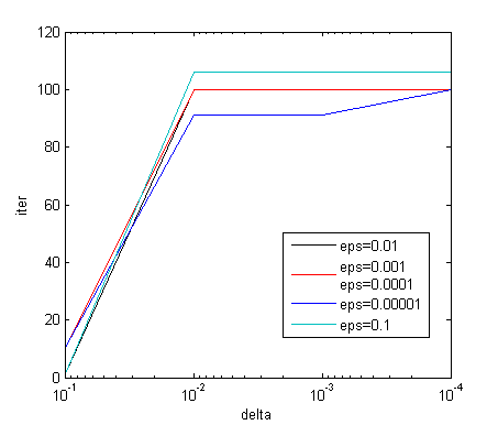 | Figure 6. Dependence of the number of iterations on parameter of precision δ |
3.4.3. Dependence of the number of iterations on parameter of parameter regularization ε
The number of iterations was measured at the fixed values of parameters α=0.04 and β=0.01. The number of iterations at different values of the parameter ε changes insignificantly, as well as at different values of precision δ.
5. Basic Conclusions Based on Numerical Results
As a result of the carried out numerical experiments it was discovered, that without boundary conditions the objective function has an endless great number of the points of minimum, located in a ravine area, that result in formal cycling of algorithm. As consequence, for providing of unicity of decision it is necessary to use boundary conditions.During numerical experiments with boundary conditions it was discovered, that:- At different precision δ the peak of number of iterations is observed at different values α. With the change of precision δ the characteristic peak of number of iterations evolves in the area of small parameters, there peak increases sharply and then it changes insignificantly.- At precision δ=0.1 the number of iterations is small. At the increase of precision to δ=0.01 the number of iterations increases sharply and then changes insignificantly. - Number of iterations at the change of parameter ε changes in the narrow range of values. As a result, it is possible to conclude that the parameter of regularization ε poorly influences on convergence of heavy-ball method.- With decrease of parameter of regularization the number of iterations of heavy-ball method rises nonlinearly.- The number of iterations at different values of parameter ε changes insignificantly, as well as at different values of precision δ.
References
| [1] | I. E. Tamm., The Bases of the Electricity Theory, Moscow: Nauka, 1989. |
| [2] | G. G. Raju, Dielectrics in electric fields, CRC Press, 2003 |
| [3] | I. A. Brigadnov, “Numerical analysis of dielectrics in powerful electrical fields”, Polish Academy of Sciences, Institute of Fundamental Technological Research, Computer Assisted Mech. Eng. Sci., Vol.8, No. 4, pp. 227-234, 2001. |
| [4] | I. A. Brigadnov, “Variational-difference method for estimation of electrical breakdown of dielectrics”, Moscow: Nauka, Math. Models and Comp. Simulations, Vol. 14, No. 4, pp. 57-66, 2002 |
| [5] | I. A. Brigadnov, “Duality method for estimation of breakdown conditions for dielectrics”, Moscow: Nauka, Math. Models and Comp. Simulations, Vol. 15, No.5, pp.106-114, 2003. |
| [6] | I. A. Brigadnov, “Duality method for limit analysis of dielectrics in powerful electric fields”, Elsevier Science Publishers B. V., J. Comp. Appl. Math., Vol.168, pp. 87-94, 2004. |
| [7] | I. A. Brigadnov, “Limit analysis method in elastostatics and electrostatics”, John Wiley & Sons, Math. Meth. Appl. Sci., Vol. 28, pp. 253-273, 2005. |
| [8] | J. Nocedal and S. J. Wright, Numerical optimization, Springer, 1999 |
| [9] | R. E. Miller, Optimization: foundations and applications, John Wiley & Sons, 2000. |
| [10] | Ch. A. Floudas and P. M. Pardalos, Encyclopedia of optimization, Vol. 2, Springer, 2001. |
| [11] | S. Attaway, Matlab: A Practical Introduction to Programming and Problem Solving, Elsevier, 2011. |
| [12] | C. B. Moler, Numerical computing with MATLAB, Cambridge University Press, 2004. |
 Abstract
 Reference
 Full-Text PDF
 Full-Text HTML