Bassem El Zoghbi
Department of Mechanical Engineering, Al Maaref University, Beirut, Lebanon
Correspondence to: Bassem El Zoghbi, Department of Mechanical Engineering, Al Maaref University, Beirut, Lebanon.
| Email: |  |
Copyright © 2019 The Author(s). Published by Scientific & Academic Publishing.
This work is licensed under the Creative Commons Attribution International License (CC BY).
http://creativecommons.org/licenses/by/4.0/

Abstract
In this paper, the damage mechanisms in unidirectional composites is investigated. The model distinguish the fiber and the matrix at mesoscopic scale. The load transfer on intact fibers neighbouring a broken fiber is evaluated. The fiber-matrix interface debonding is modelled using cohesive model in the commercial code ABAQUS. The aim of this work is to describe and analyse the micromechanics failure of carbon reinforced polyamide composites and the associated load transfer in order to predict the lifetime of such composite materials.
Keywords:
Cohesive elements, Load transfer, Unidirectional composite, Debonding
Cite this paper: Bassem El Zoghbi, Modelling of Failure Mechanism in Unidirectional Carbon Fiber-Reinforced Polyamide Composites Using Cohesive Zone Model, International Journal of Composite Materials, Vol. 9 No. 1, 2019, pp. 16-23. doi: 10.5923/j.cmaterials.20190901.03.
1. Introduction
Unidirectional fiber-reinforced polymer composites are widely used in industries due to their excellent mechanical properties such as high specific strength, resistance to corrosion and light weight. When this composite is loaded under steady loading in the direction of the fibers no macroscopic creep is recorded. However, a damage in the form of fiber failures has been detected by acoustic emission [1]. The accumulation of fiber failures could lead to premature macroscopic failure. The prediction of the service lifetime of such materials requires to understand the failure mechanisms leading to continuing fiber failure.A prematurely broken fiber leads to an overloading of adjacent fibers and in this way an increase in stress level in these fibers, which can cause a macroscopic fracture. The load transfer is defined as the ability to transfer the mechanical loading between two adjacent fibers through the surrounding matrix. Therefore, an accurate estimation of the load transfer coefficients around a broken fiber requires a detailed model of the microstructure. An understanding of the complex reality of failure phenomena was first given in 1952, by Cox [2] who considered the break of a single fibre embedded in an elastic matrix with no attempt to model the effects on the intact adjacent fibres. The main assumption of his model was that the matrix did not bear any axial load but only experienced shear loads. Hedgepeth [3] first analysed the problem of local stress concentrations using shear shear lag of stiff layers in a linear-elastic matrix. This problem was reconsidered by a large numbers of researchers using different techniques. Recently, the finite element analyses has been extensively used to model the micromechanical response of composites under longitudinal tension. S. Blassiau et al. [4] have proposed a 3D finite element model with the possibility of considering several damage states modelled by a representative volume elements R.V.E that distinguish between the fibers and matrix. In this paper, the failure mechanism will be investigated based on the R.V.E proposed by S. Blassiau et al [4]. The fibers and matrix are considered as linear elastic isotropic material. Cohesive surface elements are used to model the fiber/matrix interface permitting the interface debonding. For different states of material damage, the R.V.E is subjected to uniaxial loading in the direction of the fibers which allow us to estimate the impact of damage on the load transfer to intact fibers neighbouring a broken fiber.
2. Model Description
A microscopic scale wish distinguish the fibers and the matrix is necessary to explain the damage mechanisms in unidirectional composites. S. Blassiau et al. [4] have proposed a geometrical definition of the R.V.E based on the experimental observations of transversal cross-sections of the composite. The experimental studies [2, 3] concerning the influence of one broken fiber show that the perturbation caused is limited to the first neighbouring fibers: the intact fibers surrounding the broken fiber play a role of screen. Thus beyond the third closet fiber, it could be considered that the failure has no effect on stress filed. The retained geometries of the V.E.R represented by an elementary periodic cells are reported in Figure 1. The damage state C-S represents one broken fiber in S fibers. For example, the damage state corresponding to one broken fiber in two C-2 means that 50% of the fibers are broken and the state one broken fiber in four means that 25% of the fibers are broken, hence the reason for modelling the different states of damage in the material. The conditions of periodicity indicate a periodic break throughout the space.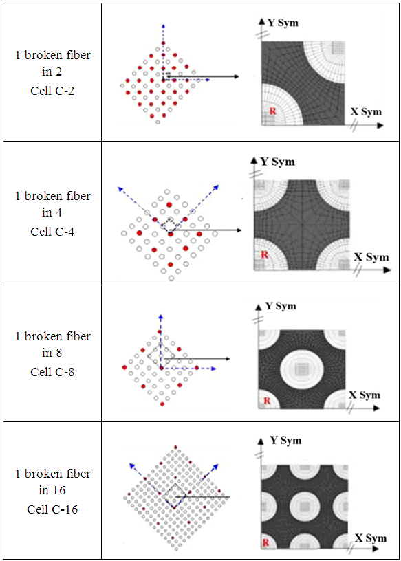 | Figure 1. R.V.E geometries of five damage states of periodic elementary cells where R represents the broken fiber [4] |
In order to investigate the damage mechanism and its development during loading, a monotonic uniaxial loading for which the interfacial decohesion, its propagation as well as the associated stress transfer are analysed. The decohesion along the fiber/matrix interface is taken into account using a cohesive zone model which is described in the following paragraph. The symmetrical nature of the problem in terms of geometry and loading allows us to consider only a quarter of a cell. The boundary conditions representing the V.E.R. under loading must represent the real loading conditions of the material and take into account the periodic microstructure. Therefore, the considered boundary conditions are the following (see Figure 2):- The displacement along x-axis ux = 0 for the nodes in the plane x = 0 which represent the geometric symmetry with respect to the plane x = 0;- The displacement along y-axis uy = 0 for the nodes in the plane y = 0 which represent the geometric symmetry with respect to the plane x = 0;- The displacement along z-axis uz = 0 for the nodes in the plane z = b/2 except the nodes of the broken fiber. These conditions represent the geometric symmetry with respect to the plane z = b/2 and the breaking of the fiber.- The periodic characteristics of the mesoscopic strain fields is represented by imposing the same displacement for the nodes in the plane x = a/2 well as the nodes in the plane y = a/2 and the nodes in the plan z = b/2.- An axial displacement is applied to the nodes in the plane z = 0 in order to simulate the field of the macroscopic uniaxial stress.The length of the cell along z-axis is adjusted to ensure a much greater length than the size of the process zone along the interface. The fiber volume fraction is taken into account by the volume of the fibers with respect to volume of the unit cell. In this study, the diameter of fibers is chosen to obtain a volume fraction of fibers about 40%.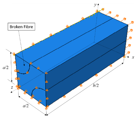 | Figure 2. Boundary conditions shown on the unit cell C-2 |
2.1. Cracking Description Using Cohesive Zone Model
The crack initiation and its propagation are described within cohesive zone methodology. The cohesive zone model is represented by a Traction-Separation law which gives the constitutive behaviour of the fracture. Abaqus offers a traction-separation model that assumes initially elastic behavior followed by the initiation and evolution of damage in composite interface. The nominal traction stress vector t acting on the cohesive element consists of 3 components: one normal component tn and two shear tractions ts and tt. The nominal strain components are defined as: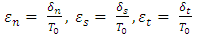 | (1) |
where  and
and  are the normal and the two shear separations, and T0 is the original thickness of the cohesive element.The available traction-separation model in Abaqus assumes initially linear elastic behavior followed by the initiation and evolution of damage. The initial elastic behavior is written as:
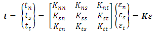 | (2) |
where Kij are the components of the elastic constitutive matrix K which represents the stiffness of the cohesive surface before damage. The damage process is activated when a criterion of failure in stress or deformation is reached. In this work, a quadratic nominal stress criterion is adopted at which the damage is assumed to initiate when a quadratic interaction function involving the nominal stress ratios reaches a value of one. The criterion is expressed as: | (3) |
where tn0, ts0 and tt0 represents the critical values of nominal traction stress components at rupture in case of pure traction or pure shear in the first and second shear directions, respectively. The Macaulay bracket  implies that a pure compressive stress does not initiate damage
  .Once the criterion of damage initiation is reached, the damage process is activated and represented by a scalar damage variable D. The initial value of D is 0 which increases with damage until it attains its maximum value 1 that corresponds to a total damage of the cohesive element. The variable damage D is specified as a tabular function of the effective displacement
  after the initiation of damage. The effective displacement
  is defined as the magnitude of the displacement vector:
 | (4) |
where  .In case of linear damage evolution, D is given by the expression proposed by Camanho et al. [5]:
 | (5) |
where  is the effective displacement at complete failure is,
  is the effective displacement at damage initiation and
  refers to the maximum value of the effective displacement during loading.The stress components are affected by the damage evolution as following:
 | (6) |
 | (7) |
 | (8) |
where  and
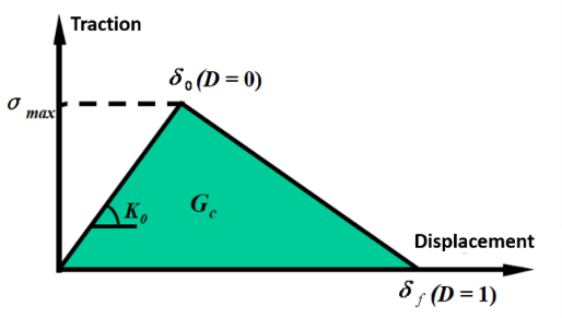
and  are the stress components calculated by the elastic traction-separation law without considering the damage. Therefore, the traction-separation response is characterized by the variation of the traction t in terms of the effective displacement
  as shown in Figure 4. The critical strain energy rate Gc corresponds to the area under the traction-separation curve.When the cohesive zone is used to model the propagation of a pre-existing crack, the simulation converge without any difficulty. However, convergence difficulties occurs if the cohesive zones are used to model crack nucleation. These problems are known to emerge from an elastic snap-back instability which occurs just after the stress reaches the maximal strength of the interface. Y.F. Gao et al. [6] have proposed a simple technique for avoiding these convergence problems by introducing a small viscosity parameter in the constitutive equations for the cohesive interface. The regularization process includes the utilisation of a viscous stiffness degradation variable Dv which is defined by the evolution equation:
 | (9) |
where  is the viscosity parameter which represents the relaxation time of the viscous system and Dv converges to the degradation variable D with time. The damage response of the viscous material becomes
 Therefore, the addition of a small value of viscosity μ compared to the time increment improves the convergence of the model in softening regime whereas the solution tends to that of the inviscid case as
  where t represents the time. However, it is must be checked if the obtained traction-separation response with such correction corresponds to the inviscid law, in particular to see if this correction does not lead to overestimation of traction and displacement.
 | Figure 3. Representation of the stress components acting on cohesive element |
 | Figure 4. Traction-Separation law of the cohesive elements |
2.1.1. Effect of Cohesive Zone Parameters on Traction-Separation Response
In this section the effect of the cohesive zone parameters on the traction-separation response is investigated by considering a case study which consists in a cohesive zone inserted between two elastic bulks subjected to simple traction as shown in Figure 5. It is known that the value of the initial stiffness of the cohesive zone should be very high in order to ensure a high stiffness of the interface before damage occurs. In order to study the effect of the stiffness on the overall elastic deformation, the stiffness of the cohesive zone is varied with a maximal traction Tmax = 50 MPa and a maximal displacement at complete failure  = 0.1 mm. For each value of K the traction-separation curve of the cohesive zone is presented in Figure 6. For K = 106 N/mm3 the obtained curve fit well with the prescribed traction-separation law, however, the elastic strain energy increases with decreasing the stiffness which leads to an adsorbed energy higher than the critical strain energy rate Gc. These results are in agreement with the empirical estimation of the minimum stiffness realized by Gonçalves et al. [7] and Camanho et al. [8] who estimated a minimum stiffness K = 106 N/mm3.
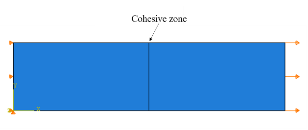 | Figure 5. Traction-Separation law of the cohesive elements |
 | Figure 6. Effect of the cohesive zone stiffness k on the traction-separation response |
In order to investigate the effect of the viscosity on the traction-separation response of the cohesive elements, we have considered several values of the viscosity  with Tmax = 50MPa, K = 106 N/mm3 and
  = 0.1mm. For each value of viscosity
  , the corresponding traction-separation curve is reported in Figure 7. The obtained results show that the levels of the maximal traction thus the amount of the adsorbed energy by the cohesive element increase with increasing the amount of the viscosity. Therefore, it is necessary to check the effect of the viscous formulation needed to converge the solution on the traction-separation response and adopt the value of viscosity
  which least disturb the traction-separation relation.In this work, a cohesive zone model is used in order to simulate the fiber-matrix debonding in unidirectional carbon fiber-reinforced polyamide composites.
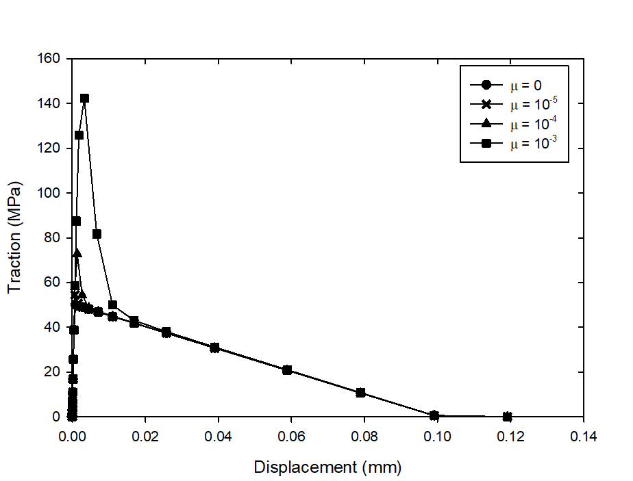 | Figure 7. Effect of the viscosity μ on the traction-separation response |
3. 3D Model of Failure Mechanism in Unidirectional Carbon Fiber-Reinforced Polyamide Composites
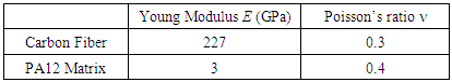
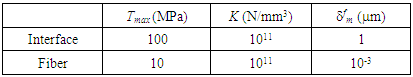
The micromechanisms of failure in fiber reinforced composite materials subjected to longitudinal tensile loading is described as follows. The fibers hold the main part of the loading and they tend to fail first. After the weakest fibers fail, the loading on remaining intact fibers increases. Then, if the fiber/matrix interface is weak, the crack will grow along the interface. The matrix cracking occurs in case of brittle matrix composites.In this work, the fibers and matrix are considered as linearly elastic materials, their elastic properties are reported in Table 1. The interfacial debonding is taken into account using a cohesive zone whose parameters are inspired by the behavior and the failure models observed in the case of amorphous solid polymers that are given in Table 2. In the case of glassy polymers, the maximum opening of the cohesive zone that corresponds to the creation of a local crack was measured by Döll, et al. [9, 10] using optical interferometry, its magnitude is of the order of 1-10μm. The interface involving a polymer-metal bond for which the polymer phases damages, a maximal displacement at failure  = 1μm is adopted. The traction at the initiation of the decohesion is considered to be of the same order of magnitude as the tensile strength of the polyamide PA12.
Table 1. Elastic Properties of Fiber and Matrix
 |
| |
|
Table 2. Cohesive Zone Parameters of Broken Fiber and Fiber/Matrix Interface
 |
| |
|
In order to have a crack that starts to propagate at the fiber and then passes into the fiber-matrix interface, a cohesive zone is inserted into the broken fiber whose properties are given in Table 2. The low value (Tmax = 10 MPa) of the decohesion stress of the fiber indicates that its rupture will take place from the first moments of loading and will be followed by interface debonding. This is motivated by our interest in decohesion analysis during load transfer.The fiber/matrix interface is meshed with 8-node three-dimensional cohesive elements COH3D8. Mesh partitions are made for the fiber and matrix adjacent to the interface, so that the neighboring parts of the interface are meshed with 8-node linear brick elements C3D8 having the same dimensions as the elements of the interface (see Figure 8).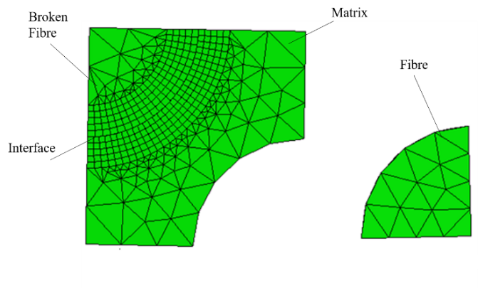 | Figure 8. Mesh |
3.1. Composite without Damage
The mechanical response of the composite without damage is considered by applying a macroscopic deformation of 2% in order to find the global stress-strain curve for the cell as well as for the fiber and the matrix. The variation of the maximum main stress (axial strain) in terms of the macroscopic deformation in the carbon fiber, in the matrix and in the whole cell are reported in Figure 9. The same response is obtained for all intact cells because the conditions of periodicity as well as the volume fraction of fibers are respected for all cells (C-2, C-4, C-8 and C-16).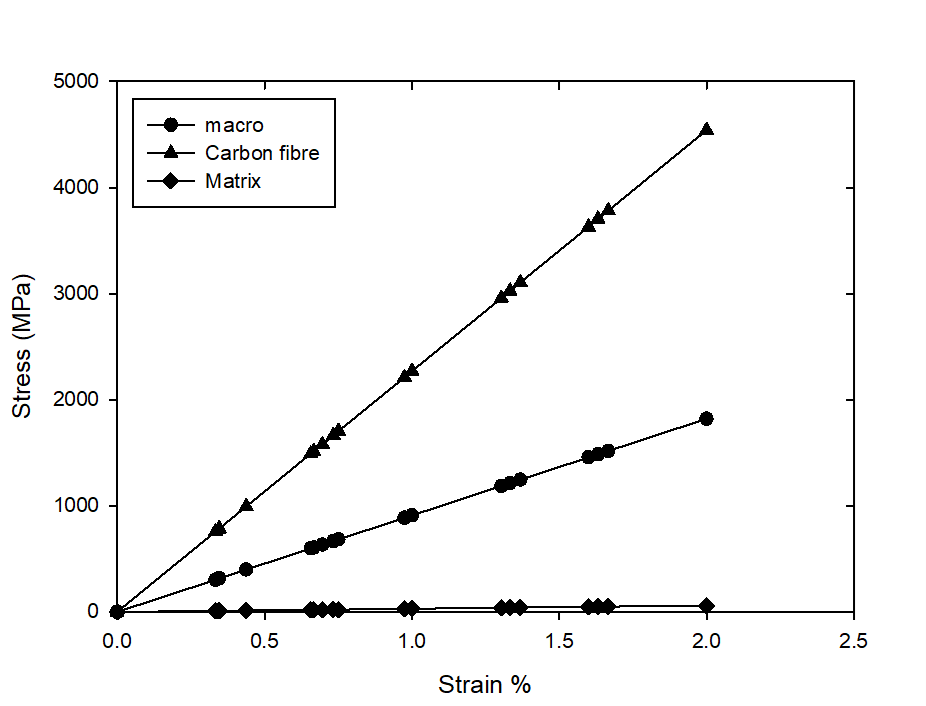 | Figure 9. Variation of the macroscopic axial stress versus the macroscopic axial strain during loading |
3.2. Coefficient of Load Transfer
The purpose of this calculation is to simulate a fiber failure and to describe the evolution of the stresses in neighboring fibers as a function of time, versus distance from the plane of failure. This evolution is quantified by the calculation of the load transfer coefficient k which is defined from the calculation of the mean of the axial stress in the considered fiber between two consecutive sections of the mesh, divided by the same amount in the intact configuration. Therefore, the coefficient of load transfer is given as 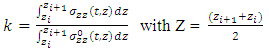 - t is time of loading which represents the imposed axial strain;-
  is the axial stress in the fiber;-
  is the axial stress in the fiber of the intact material;- Zi+1 and Zi are the abscises of the cross-sections where the mean stresses are calculated.
3.3. Configurations C-2, C-4, C-8 and C-16
In this section, the results related to configuration C-2, C-4, C-8 and C-16 are represented. The mechanical properties of the interface are Tmax = 100 MPa and  = 1 μm. The composite is strained in the fiber axis direction, the same velocity is applied for all configurations. A viscosity parameter of cohesive elements μ = 0.01 for cohesive elements of all configurations is used in order to avoid the convergence problems.
3.3.1. Observation of Damage during Loading
In order to illustrate the damage propagation during loading, the distribution of damage variable D (denoted SDEG into Abaqus) for different load levels are reported in Figure 10. The initial value of D is 0 which increases with damage initiation until it attains its maximum value 1 when a local crack takes place. Figure 10 shows that the damage begins from the plane of the broken fiber at the beginning of the loading then the crack propagates progressively along the interface during loading. The cracked zone is followed by an intermediate zone where the damage variable D varies between 0 and 1 corresponding to the extent of the process zone which is well distributed over several elements and its size is much smaller than the length Z of the cell. From these results, the load transfer to intact neighboring fiber is analyzed.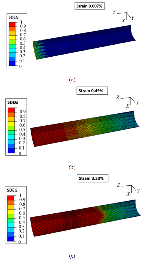 | Figure 10. Distribution of the damage variable SDEG of the cohesive elements along the broken fiber/matrix interface during loading (SDEG = 0 corresponds to no damage and SDEG = 1 corresponds to a local crack) |
3.3.2. Load Transfer during Loading
The variation of the main stress  along the intact closest fiber to the broken fiber during loading is shown in Figure 11. During decohesion, the maximum main stress is always located in the vicinity of the plane of rupture of the first fiber. Its level increases during loading.
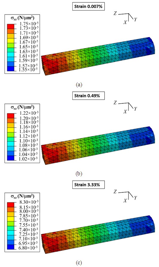 | Figure 11. Distribution of the principal stress σzz along the intact closest fiber to the broken one during loading |
By comparing the macroscopic response of the undamaged and damaged composite materials, it shows that the rigidity of the composite material decreases with damage. This observation raises the question of the definition of the reference state to be chosen: either the stress distribution should be compared with the undamaged case for the same macroscopic strain or for the same macroscopic stress.As our loading conditions are defined with imposed deformations, the reference state is considered that of undamaged cell with same macroscopic strain. However, it seems appropriate to impose the deformation and to let the stress distribution takes place in order to evaluate the load transfer in stress on the nearest intact fibers. The choice of comparing the undamaged and damaged states with identical macroscopic stress was adopted by S. Blassiau et al. [4]; by invoking the fact that a problem in creep was considered. In the case of an undamaged cell, the two approaches are equivalent. However, when the damage appears, the comparison with identical macroscopic deformation seems to us more realistic. The load transfer coefficients k for cells C-2, C-4, C-8 and C-16 in the nearest fiber to the broken fiber in terms of the distance Z from the plane of failure (Z = b/2 = 28.5μm) for different levels of the macroscopic deformation are reported in Figure 12. The shape of load transfer curve along the nearest intact fiber to the broken fiber of all configurations is similar where the maximum load is located in the region close to the plane of failure. However, the magnitude of the load transfer coefficient decreases with the broken fiber rate in the VER, the maximum of k going from 1.1 for C-2 to 1.04, 1.02 and 1.01 for the configurations C-4, C-8 and C-16 respectively. In fact, the load transfer is distributed on the nearest intact fiber but also on the other intact fibers, then the magnitude of the load transfer coefficient decreases with increasing the rate of broken fibers. 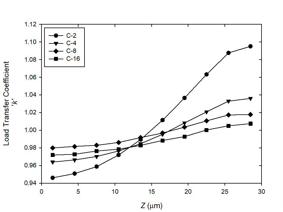 | Figure 12. Load transfer coefficient k in the nearest fiber to the broken fiber in terms of the distance Z from the plane of failure (Z = 28.5 μm) for cells C-2, C-4, C-8 and C-16 with a reference state at same macroscopic strain |
These results show that the highest magnitude of the load transfer generated in the intact fibers of a damaged R. V. E is 1.1 for the configuration C-2 with 50% of broken fibers. This estimation is notably lower than that predicted by S. Blassiau et al. [4] for a similar configuration where k ranged from 1.4 (without interfacial decohesion) to 2 (with considering the interfacial decohesion). In fact, the difference comes from a distinct reference state depending on whether a reference intact state with identical macroscopic deformation or stress is considered.By taking as reference state an intact material subjected to identical macroscopic stress, a load transfer coefficient k about 2 is predicted for the configuration C-2 (see Figure 13). This value of k is similar to that obtained by S. Blassiau et al. [4].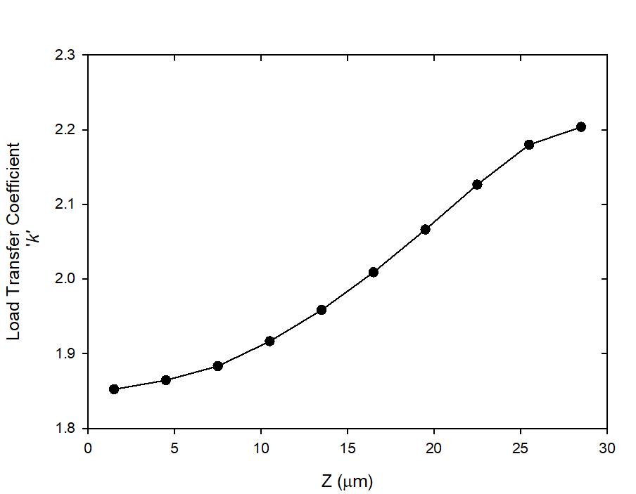 | Figure 13. Load transfer coefficient k in the nearest fiber to the broken fiber in terms of the distance Z from the plane of failure (Z = 28.5 μm) for cell C-2 with a reference state at same macroscopic stress |
Therefore, the definition of the intact reference state appears important in the evaluation of the load transfer coefficient k.
3.4. Influence of the Characteristics of the Interfacial Cohesive Zone on the Prediction of the Load Transfer Coefficients
The aging of the polymer matrix of the composite materials is manifested by a reduction of the deformation at break  of the matrix by a factor of 2 essentially due to a cleavage of the chains. From a mechanical point of view, this effect can be manifested by:- a reduction of the maximal displacement
  being correlated with the deformation at break
  ,- a reduction of the maximal tension Tmax which represents the decreasing in the interfacial bonding rate due to the rupture of the chains of the polymer matrix.In order to evaluate the influence of each of these two effects, a parametric study on the influence of the characteristics Tmax and
  of the interfacial cohesive zone on the load transfer coefficient is evaluated by considering a reduction of 50% in
  then by a reduction of 50% in Tmax and finally by considering a reduction of 50% in both
  and Tmax. For each of these cases, the distribution of the load transfer coefficient along the nearest fiber to the broken fiber in terms of the distance Z in cell C-2 are evaluated at same macroscopic deformation. The obtained results are shown in Figure 14. The values of Tmax = 100MPa and
  = 1μm are considered as reference case. The results do not show any significant influence on the load transfer k. This latter is sensitive to the variation of rigidity than the phenomenon of decohesion. Therefore, the values of Tmax and
  govern rather the rate of damage in composite materials rather than the load transfer at a fixed percentage of broken fibers.
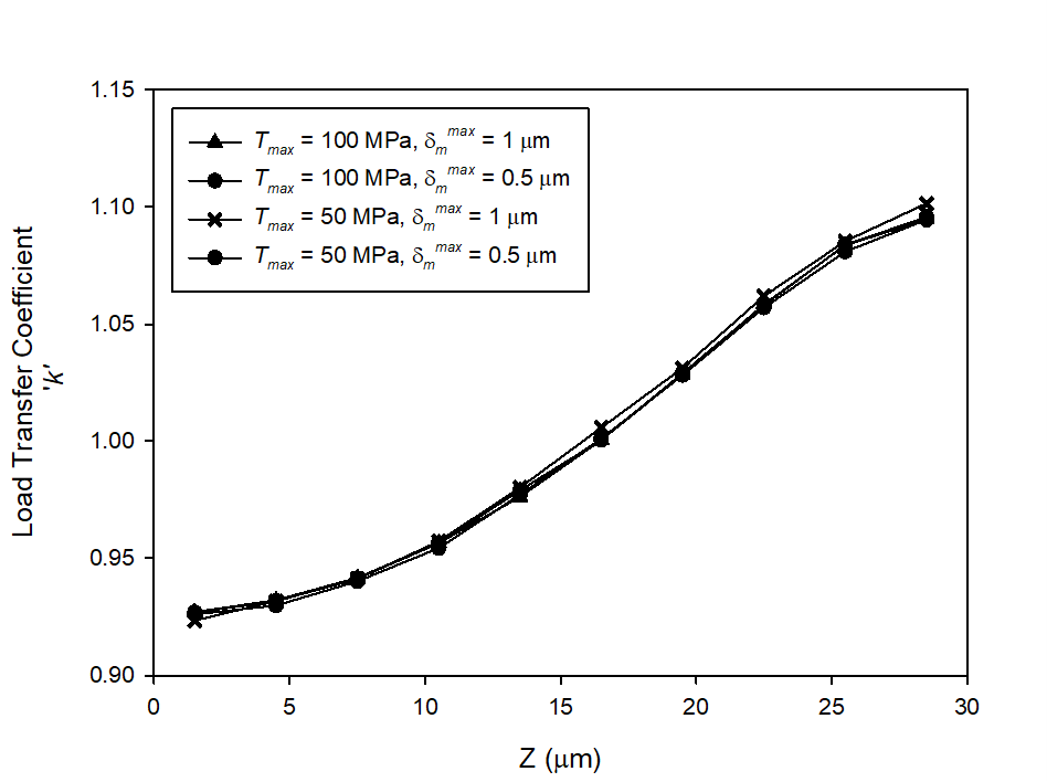 | Figure 14. Load transfer coefficient k in the nearest fiber to the broken fiber in terms of the distance Z from the plane of failure (Z = 28.5 μm) in cell C-2 according to the cohesive zone characteristics (Tmax ,  ) ) |
4. Conclusions
In this work, a finite element analysis of the micromechanical damage of unidirectional fiber-reinforced carbon polyamide composite is presented. The mechanisms of damage are performed by a cohesive zone model whose characteristics are physically realistic. The methodology of analysis with the definition of the V.E.R representing different states of damage in the composite are presented. The loads transferred from a fiber damaged by rupture then by interfacial decohesion to the intact neighbouring fibers are evaluated. The load transfer coefficient is predicted by comparing the stress distribution along the closest intact fiber to the broken fiber in the damaged R.V.E and that in the intact configuration for identical macroscopic deformation. The model has confirmed that the increasing of the rate of broken fiber leads to an increasing of the rate of load transfer. The definition of the intact reference state depending on whether a reference intact state with identical macroscopic deformation or stress is shown important in the evaluation of the load transfer coefficient k. The effect of aging in composite materials manifested by a reduction of cohesive characteristics (Tmax and  ) do not show any significant influence on the prediction of the load transfer coefficient which is sensitive to the variation of rigidity more than the phenomenon of decohesion.
References
| [1] | Bunsell AR, Fuwa M. An acoustic emission proof test for a carbon fibre reinforced epoxy pressure vessel. In: Eighth world conference on non-destructive testing, 1976. p. 1–8. |
| [2] | H. L. Cox, The Elasticity and Strength of Paper and Other Fibrous Materials, British Journal of Applied Physics, Vol. 3, No. 3, 1952, p. 72-79. |
| [3] | Hedgepeth JM. Stress concentrations in filamentary structures. NASA TND-882, Langley Research Center, 1961. |
| [4] | Blassiau, S., Thionnet, A., Bunsell, A.R., 2009. Three-dimensional analysis of load transfer micro-mechanisms in fibre/matrix composites. Compos. Sci. Technol. 69 (1), 33–39. |
| [5] | Camanho, P. P., and C. G. Davila, “Mixed-Mode Decohesion Finite Elements for the Simulation of Delamination in Composite Materials,” NASA/TM-2002–211737, pp. 1–37, 2002. |
| [6] | Y. F. Gao and A. F. Bower, “A Simple Technique for Avoiding Convergence Problems in Finite Element Simulations of Crack Nucleation and Growth on Cohesive Interfaces,” Modelling and Simulation in Materials Science and Engineering, Vol. 12, No. 3, 2004, pp. 453-463. |
| [7] | Goncalves, J., De Moura, M., De Castro, P. and Marques, A., Interface element including point-to-surface constraints for three-dimensional problems with damage propagation. Engineering Computations, Vol. 17, No. 1, 28-47, 2000. |
| [8] | Camanho P.P., Davila C. G., de Moura M.F., "Numerical simulation of mixed-mode progressive delamination in composite materials," J Compos Mater, vol. 37, no. 16, pp. 1415-1438, 2003. |
| [9] | Döll W. (1983) Optical interference measurements and fracture mechanics analysis of crack tip craze zones. In: Kausch H.H. (eds) Crazing in Polymers. Advances in Polymer Science, vol 52-53. Springer, Berlin, Heidelberg. |
| [10] | Döll W., Könczöl L. (1990) Micromechanics of fracture under static and fatigue loading: Optical interferometry of crack tip craze zones. In: Kausch H.H. (eds) Crazing in Polymers Vol. 2. Advances in Polymer Science, vol 91/92. Springer, Berlin, Heidelberg. |

 Abstract
 Reference
 Full-Text PDF
 Full-text HTML