1. Introduction

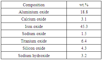
Red mud is the residual waste produced from the production of alumina from bauxite (Bayer Process) and is obtained during the digestion process in which sodium hydroxide (NaOH) is added to the bauxite. The Bayer process is the most economical process for the gibbsitic type of bauxite found in Jamaica, particularly as it contains large quantity of Fe₂O₃ [1]. Red mud may be described as a mineral waste, composing of hematite (Fe₂O₃), left-over aluminium oxide (Al₂O₃), silica (SiO₂), some titanium dioxide (TiO₂), sodium hydroxide (NaOH) and other residual minerals [2]. The addition of sodium hydroxide makes the red mud highly alkaline (usually pH 10 to 14). Parekh and Goldberger [3] described red mud as being clay-like in nature because of its iron content, which usually imparts a red colour to the waste.

The steady increase in aluminium production worldwide is a concern due to the subsequent escalation in the amount of red mud that has to be disposed of, considering that every tonne of alumina produced in Jamaica results in the production of ~1.5 tonnes of red mud. Data obtained from the Jamaica Bauxite Institute have shown that between 1990 and 2004 over 76 million tonnes of red mud were released to man-made lakes or ponds, and most of these lakes have either been abandoned or are operating beyond their threshold levels. Tsakiridis et al. [4] reported that a 5-million tonne per year alumina plant requires approximately 100 hectares (247 acres) of land per year for disposing the red mud, which is often prime agricultural land in Jamaica. This is significant and poses a scarcity in available land space, considering that Power et al. [5] estimated that about 2.4 billion tonnes of red mud are stored globally.

Red mud is environmentally harmful due to its fine particle size and high caustic content. It can impact negatively on the surrounding communities, especially in Jamaica where people live close to the storage sites. In addition to dust problems, red mud may seep into underground water supply or flow into nearby tributaries and rivers [3, 6], and this can have serious consequence on humans and livestock, as well as adverse effect on the physical and ecotoxicological properties of soil and plant, respectively. The storage solution is also economically problematic due to the high cost of maintenance of containment structures to prevent leaching [7].

The problem of reducing the amount in storage is a challenge, and numerous studies have been undertaken to explore viable potential application of red mud. Sutar et al. [1] reviewed a number of strategies that are currently employed to reduce the stockpile of red mud, such as in the manufacture of building materials and composites, soil amendment, catalysis, adsorbents, metal recovery, and neutralization. The production of building materials (brick, tile, roofing and cement) [8-12] and glass and ceramic [13-15] were the focus of early studies. For example, Wagh [10] manufactured bricks by using sodium silicate as the binding agent instead of the traditional firing method. The bricks were made from 100% untreated red mud, sieved to finer particle sizes as these showed higher compressive strengths. Rudraswamy and Prakash [16] also showed that a replacement level of 10% red mud in ordinary Portland cement resulted in increased tensile, compressive, flexural, and shear strength, irrespective of whether the red mud was washed or unwashed. When compared with 100% cement, the lowest increased was 2.8% in compressive strength (washed) and the highest was 27.1% in flexural strength (unwashed). It should be noted that according to Thakur and Sant [17], the sodium alumina silicate in red mud is a good bonding property and could have contributed to the improved strength. Sglavo et al. [15] investigated the use of red mud as a component in clay mixtures for ceramic production, and found that a red mud/clay mixture, under specified conditions, yielded increased density and flexural strength in the final product as a result of the formation of a glassy phase.

Red mud has also been used as a filler for natural fibre and polymer reinforcement to improve the physical and mechanical [18-21], electrical and thermal conductivity [14, 22, 23], and tribological properties [24, 25]. For example, Saxena et al. [13] developed a new composite building material using industrial waste (red mud and fly ash) and natural fibre (sisal and jute) in a polymer matrix. The study revealed that the developed product, in comparison to conventional wood-based products, attained superior mechanical, physical and chemical properties. More recently, Prabu et al. [21] fabricated red mud composites reinforced with natural fibres and polyester, and the results showed that the addition of red mud promotes a marginal increase in the mechanical strength.

Other studies have shown that red mud is compatible with polymers as well as other binding agents like cement. In that vein, the present study present study seeks to investigate the properties of a recycled polymer-red mud composite with the main objective of developing the mathematical relationship between the properties of the composite and the influential control factors and interactions.

2. Materials and Methods

2.1. Preparation of Composite

Red mud (pH 14) was obtained from the red mud lake and flocculation tanks at the Kirkvine Alumina Company in Mandeville, and the nominal as-received composition is shown in Table 1. The red mud was then dried in an oven at a temperature of 105°C for 24 hours, crushed and sieved to two particle sizes, ASTM 80 and 40 mesh (180 and 425 µm).

Both samples were mixed with dilute HCl and then filtered to remove the sodium hydroxide, and again washed with distilled water until pH 7 was obtained, dried, crushed, and sieved to their previous particle size.

The samples were mixed with recycled high-density polyethylene (HDPE) pellets to different ratios. Prior to mixing, the HDPE pellets were coated with a mixture of lubricating oil and vegetable oil in the ratio of 60:40, which comprised 6 wt.% of the total mixture. The mixture of red mud, polymer and oil was first placed in a hot mixer at a temperature of 175°C until the polymer was liquefied and properly mixed with the red mud. Afterwards, the mixture was immediately transferred to an encapsulator where it was uniaxially compressed at 20 MPa for 10 minutes in a 25-mm diameter mould until it was cooled by natural convection. The sample was then removed from the mould and stored in moisture-proof container for testing.

Table 1. Nominal Composition (wt.%) of the As-Received Red Mud

2.2. Design of Experiment

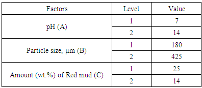
A full factorial design of experiment of the type p^k was used in this study, where “p” and “k” represent the number of levels and factors, respectively, and these are shown in Table 2. Three two-level factors, pH (A), particle size (B), and amount of red mud in the composite (C), were selected as the independent variables. The as-received pH of the red mud was 14 but was treated to reduce the pH to a neutral value. Hence, pH of 7 and 14 were used as Level 1 and Level 2, respectively. The two sieve sizes (fine and medium) used in the study were 180 and 425 µm, and the amount of red mud in the composite was set at 25 and 75 wt.%. These were chosen so that the effect would be as apparent as possible.

Table 2. Experimental Values of the Factor-Levels

Table 3 shows the experimental design for each test. The number of experiments for a full factorial design is 8; however, each experimental design will be replicated, hence, 16 samples were prepared.

The density and hardness were first determined following standard laboratory procedures. The hardness was measured by a Brinel hardness tester.

Table 3. Design of Experiment and Results of Hardness and Density Tests

A polynomial linear regression model was used to represent the relationship between the predicted outcome variables (hardness and density) and the predictor variables (factors and their interactions). This model was first considered as linear behaviour usually occurs in physicochemical analysis of ingredients mixture [26]. For the experimental design used in this study, the general form of the model is expressed as:

(1)

where Y is the predicted outcome variable, b₀ is the intercept of the regression equation, b₁ to b₆ are the regression coefficients, and A to BC are the predictor variables.

The Analysis of Variance (ANOVA) was used to investigate the effects of the factors and interactions, as well as their relative contribution to the precision of the model. The ANOVA was carried out on the model for a confidence level of 95% (p ≤ 0.05). The factors and interactions that showed a significant effect were then used to obtain the final regression model. In order to ensure that the goodness of the fit of the regression model was obtained, the test for significance of the model, the analysis of the residuals, and the test for lack of fit were performed [27]. All analyses were done by using the software Statistica.

3. Results and Discussion

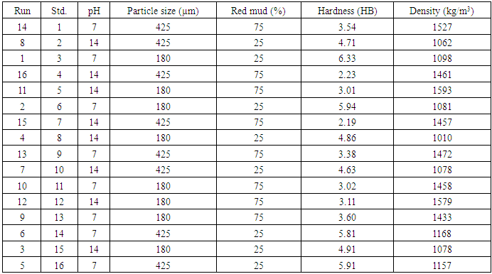
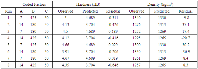
The results of the hardness and density of the 16 runs on the red mud/polymer samples are shown in Table 3. The initial linear regression model, showing the coded relationship between the predicted outcome variables and the predictor variables are as follows:

(2)

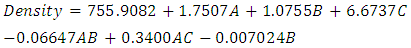(3)

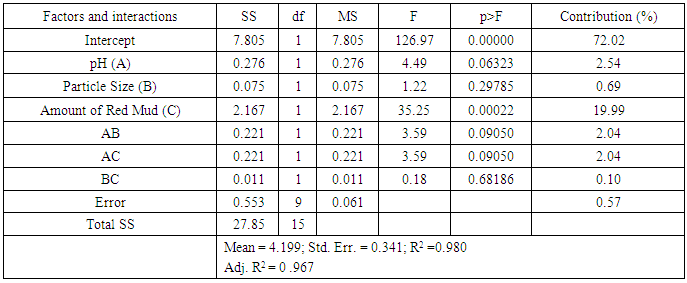
3.1. Analysis of Variance

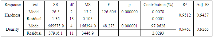
The results of the ANOVA for the initial regression model for the hardness of the composite are presented in Table 4. Examination of the table shows that only the amount of red mud has a significant influence on the hardness of the composite, as p is less than 0.05 (i.e., α = 0.05 or 95% confidence). Also, the interactions (AB, AC, and BC) did not influence the hardness. The last column in Table 4 shows the degree of contribution of the factors and their interactions to the hardness, and it can be seen that the amount of red mud (19.99%) and the pH (2.54%) are the major factors influencing the hardness. The dominant effect of the amount of red mud can be attributed to its low shear strength when compared to the HDPE. Additionally, the error contribution is 0.57%.

Table 4. ANOVA Table for Testing the Significance of Regression Model for Hardness

The results of the ANOVA for the density of the composite are presented in Table 5. Here, the particle size and the amount of red mud are both considered to be the statistically significant factors that influence the density of the composite, contributing 18.36% and 13.17%, respectively, to the model. Furthermore, all the main effect interactions considered in this study are statistically significant as their p value is less than 0.05.

Table 5. ANOVA Table for Testing the Significance of Regression Model for Density

The interaction between pH and amount of red mud is the predominant interaction contributor (9.40%) to the model, and closely followed by the interaction effect of pH and particle size (8.63%), with the error contributing only 0.67%. Therefore, it is evident that the proposed model should contain two factors (B and C) and the interactions (AB, AC and BC).

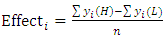
3.2. Estimates of Main Effects

The effect of a factor is the average response when the factor changes from one level to another level. In this study, the main effect of a factor is the change in the predicted outcome from the low level to the high level, and is calculated using the equation:

(4)

where ∑y_i(H) and ∑y_i(L) are the sum of the runs at the high and low level, respectively, for each factor, and n is the number of data collected at each level. Thus, from Table 3, the following are the calculations for the main effect of pH on the hardness.

Therefore, .

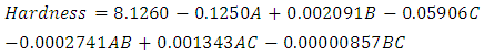
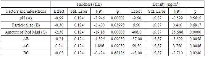
The estimates of the main effects of the factors and interactions were calculated using ANOVA and are presented in Table 6. It can be seen that the amount of red mud and pH are the two major factors that have markedly affect the hardness of the composite. Here, the mean hardness of the composite decreases by 2.38 HB when the amount of red mud in the composite is changed from 25 to 75% while maintaining the same level for the other factors. On the other hand, if the setting factor was changed for pH with the other factors kept constant, the hardness would only decrease by 0.99. The decrease of the pH from 14 (high) to 7 (low) causes a markedly increase in hardness, and this can be attributed to the method used to treat the as-received red mud, which probably allowed the binding constituents in the red mud to be in intimate contact. In an early study, Thakur and Sant [17] stated that the sodium alumina silicate in red mud is a good bonding property, and the drying of the red mud would allow the sodium alumina silicate to come together and bond, thereby increasing the resistance to flow.

Table 6. Effect Estimates of Factors and Interactions Resulting from Change in Level

Table 6 also shows that the change in the amount of red mud has the greatest effect on density, which is expected to increase by 406.0 kg/m³ when the percentage of red mud is changed from 25 to 75%. The main effects of the other control factors, pH and particle size, are minor but the values may be misleading owing to the main effects of the interactions.

3.3. Development of the Model

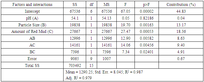
It is observed in Tables 4 and 5 that the coefficients of determination, R², of the initial model for hardness and density are 98.0 and 98.7%, respectively. R² is defined as the ratio of the explained variation to the total variation and may be interpreted as a measure of the degree of fit [28]. The values of R² are close to unity, which indicate that a model can be built that should provide satisfactory predictable outcomes. A high R², nevertheless, does not necessarily indicate that the model is adequate. For that reason, a lack of fit test was performed on Equation 2 and 3, and the p-values obtained were 0.0207 and 0.0231, respectively. Hence, at 95% confidence, the models are inadequate, and must be improved by removing insignificant factors and interactions. In addition to the lack of fit test, the improved models will also be checked by analyzing the residuals of the models.

Using the significant factors and interactions, as well as the major contributors, we arrive at the revised regression model for each predicted outcome in terms of the coded factors.

(5)

(6)

Equation 5 indicates that, within the range of the experiment, the hardness of the composite is reduced with higher levels of pH and amount of red mud. This agrees with the negative values of the effect estimates given in Table 6. For Equation 6, the terms with the positive coefficients increase the density while those with the negative terms have an opposite effect.

3.4. Checking the Adequacy of the Developed Model

The summary of results of the analysis for the revised models is shown in Table 7. The F-ratios of the models were determined by ANOVA and found to be adequate at 95% confidence. Particularly important is that the error contributions are 0.0078 and 2.03% for the hardness and density, respectively. The lower percentage error in the hardness of the composite suggests that it can be predicted more accurately than the density, and this can be attributed to the larger number of terms in Equation 6.

Table 7. Test of Model vs Residual

The goodness of fit of the models was also tested by R² and the adjusted R². Here, R² is the proportion of variance in the observed values of hardness and density values that is accounted for by the factors and interactions in the regression model, while the adjusted R² makes adjustment for the number of factors and interactions in the model. For hardness, R² and the adjusted R² are 95.12 and 94.37%, respectively, while for density, the values are 94.61 and 92.65%, respectively. The adjusted R² may decrease if the factors and interactions entered in the model do not add significantly to the model fit. In these models, the reduction is negligible; therefore, the terms in the models are appropriate.

The normal probability plots of the residuals for both the hardness and density are shown in Figures 1 and 2, respectively. The residuals are the differences between the observed (measured) values and predicted values, and the expected normal value is the standardized z-values of the normal distribution. It can be seen that the residuals generally fall on a straight line implying that the errors are normally distributed [29]. Hence, the regression models appear to be suitable in predicting the correct responses.

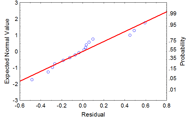Figure 1. Normal probability plot of residuals for density

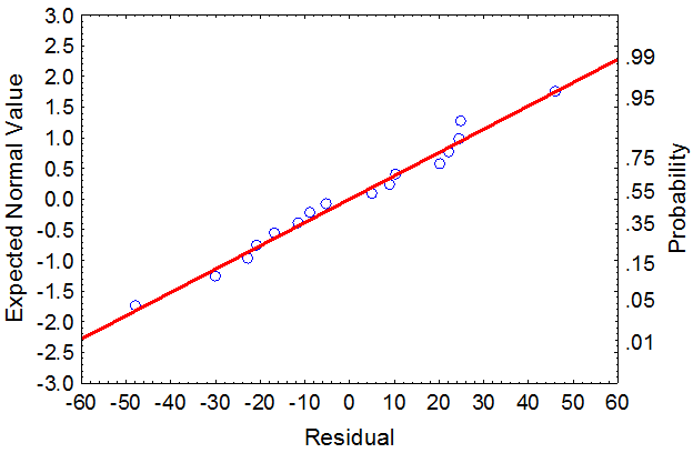Figure 2. Normal probability plot of residuals for hardness

Figures 3 and 4 show the plots of the studentized residuals against the predicted values. The plots, however, do not exhibit random scatter of the residuals, but this is expected. Figure 3 shows a definite pattern with four vertical lines (represented by unfilled circular markers) that correspond to the four possible predicted values from Equation 5, the two levels of the two factors, A and C; that is, 2 × 2 = 4. The scatter of residuals within each vertical line represents the variability in the group, but the variations are acceptable as all the studentized residuals are within the ± 2 (± 97.72%) limits. In Figure 4, while the residuals are within the ± 2 limits, the lines appear to be confined to two vertical zones, which is indicative of the importance of the two levels of factor C to Equation 4. Again, this is not surprising as the contribution of factor C was most influential (94.81%) in the initial development of the model (see Table 5).

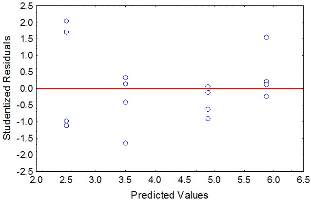Figure 3. Plot of predicted values vs studentized residuals for hardness

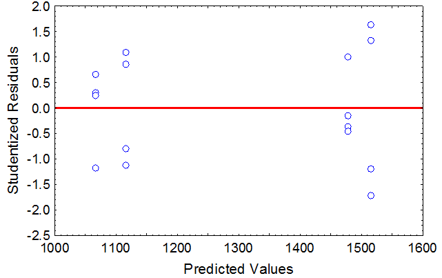Figure 4. Plot of predicted values vs studentized residuals for density

3.5. Validation of Models

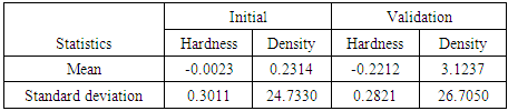
To check the adequacy of the revised mathematical models eight experimental runs were conducted, and the new data were used to compare with the predictions of the revised model [30]. The experimental design for the validation and the subsequent results are shown in Table 8. The table also shows the values predicted by the revised models (Equations 5 and 6) and the residuals. The mean and standard deviation of the residuals from the initial and validation runs are presented in Table 9. Statistically, for a 95% confidence, there is no significant difference between the distributions of the residuals of both runs for the hardness and density, as the calculated p-values were 0.1101 and 0.7948, respectively. Therefore, these results indicate that the predictive strength of both models is satisfactory.

Figures 5 and 6 show the plots of the predicted and observed values of hardness and density for the validation runs. The reason for the vertical circular markers in the figures (two in Figure 5 and four in Figure 6) is similar to the explanation given earlier for Figures 3 and 4. More importantly, the residuals are generally with the 95% confidence limit, which indicate the validity of the models.

Table 8. Design of Validated Runs and Results

Table 9. Descriptive Statistics of Residuals for Initial and Validation Runs

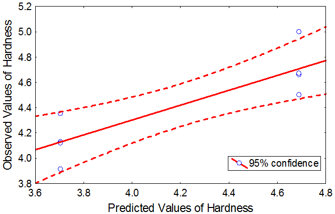Figure 5. Plot of predicted and observed values of hardness (HB), showing residuals, R = 0.864

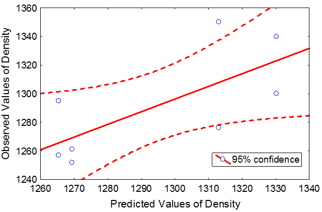Figure 6. Plot of predicted and observed values of density (kg/m3), showing residuals, R = 0 .706

4. Conclusions

The present study has used a full factorial design of experiment to develop multiple linear regression equations for predicting the hardness and density of different combinations of polymer-red mud composite, based on the pH, particle size, and the amount of red mud. ANOVA was used to determine the significant factors and interactions for the models at the 95% confidence level, and the adequacy of the models was tested using goodness of fit test and scatter diagrams, after which the models were validated with a new set of data that were within the ranges of the experimental factors. The results from the validation experiments showed that the developed models are reasonably accurate in predicting the hardness and density of the polymer/red mud composite.