1. Introduction

Liquid composite molding (LCM) is one of the most popular composite manufacturing processes due to its repeatability, medium costs, and flexibility. Resin is injected or infused into a mold filled with dry fabric, this process is performed under different conditions (constant pressure or velocity, atmospheric or vacuum outlet ports…) with different methods such as RTM, VARTM, VARI, and RIFT.

In order to simulate the resin injection and to predict the filling time of any structure, the permeability of the fabric is required. A dry fabric is considered as a dual scale medium, Figure 1. Researchers classify the flow inside the bundles as “microscopic flow”, between the bundles as “mesoscopic flow”, and as “macroscopic flow” at piece level. In other words, the permeability of bundles or unidirectional yarns is called microscopic permeability while that for a fabric is called macroscopic permeability. Microscopic permeability is an important parameter to discover resin flow through the fiber bed and understand the mechanisms of air entrapment which governs the quality of composite parts made by LCM. Moreover, it is an essential step towards macroscopic permeability modeling.

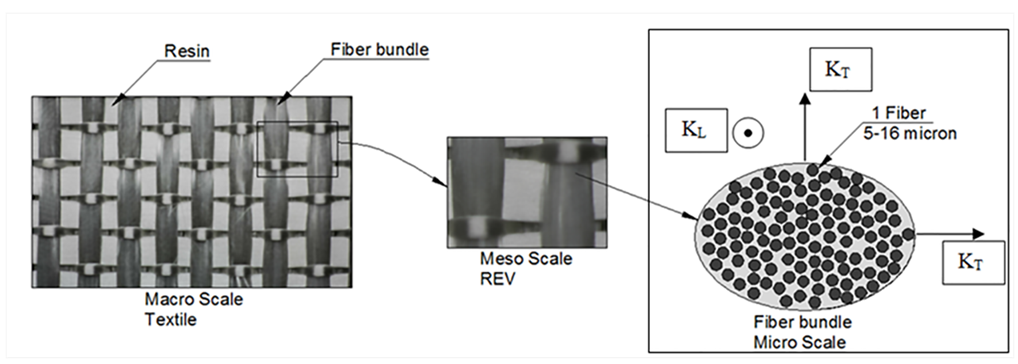Figure 1. P3W-GE044 from 3TEX Company

1.1. Problem Statement

This study deals with microscopic permeability of unidirectional yarns; longitudinal permeability K_L and transverse permeability K_T. In general, the evaluation of these permeability values is done by experimental measurements, analytical models, or finite Element (FE) numerical simulations. While analyzing the previously stated prediction methods, wide scattering is observed. In addition, many analytical models exist, while there is no clear comparative study that evaluates all these models.

The main objective of this paper is to evaluate the available analytical models, by comparing their results to the available bibliography data. However, because of the wide scattering found in bibliography results, this data is to be refined. Thus a finite element modeling is done, in which a more realistic unit cell is used where the fibers are arranged in a random manner; neither square nor hexagonal. Static mode and transient mode simulations are launched. The values of transient simulations approved the consistency of static mode simulations. The bibliography results that better fit the FE modeling results are selected. Then a comparative study is performed and the best analytical models for K_L and K_T are presented.

1.1.1. Bibliographic Experimental and Numerical Scattering

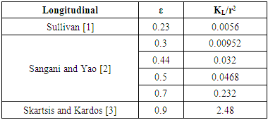
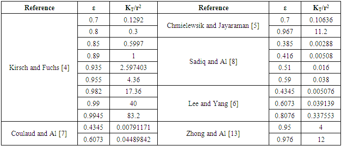
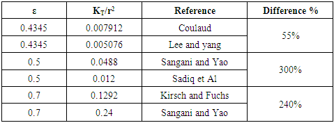
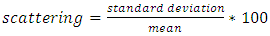
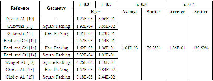
Researchers [1-12] predicted the permeability values either by numerical simulations or experimental measurements. This section aims to show the scattering found for both experimental measurements and numerical predictions for aligned fiber beds with the same fiber volume fraction. Permeability measurements depend on many parameters including the method, the apparatus, the techniques and operator skills, as well as the injection method which could be either radial or unidirectional. On the other hand, numerical simulations depend on many parameters such as the used code, the used method, the boundary conditions, and the most important and influencing parameter which is the unit cell selection. Table 1, Table 2, and Table 3 show different experimental measurements and numerical simulations of the dimensionless permeability components K_L/r² and K_T/r² values, where “r” is the fiber radius.

Table 1. Measurements for longitudinal microscopic permeability

Table 2. Measurements for transversal microscopic permeability

Table 3. Permeability values with corresponding scattering

Sullivan [1] measured the permeability for different fiber types like glass wool, goat wool, and copper wire, with cross sectional diameter ranging from 7.6µm up to 150.5µm. Sangani and Yao [2] predicted the permeability of aligned cylinders in different array structures. Skartsis and Kardos [3] measured the permeability and consolidation of oriented carbon fiber beds. Concerning transversal permeability, Kirsch and Fuchs [4] performed a permeability study on fibrous parallel cylinders of aerosol filters which consist of kapron fibers of diameters 0.15, 0.225 and 0.4mm. Chmielewsik and Jayaraman [5] measured experimentally the transversal permeability for acrylic circular cylinders array having a diameter of 4.76 mm and 38 mm long. Coulaud and Al. [7] chose a numerical method where the medium has been modeled by cylinders of either equal or unequal diameters arranged in a regular pattern with a square or triangular base. Sadiq and Al. [8] measured the transversal permeability of unidirectional cylinders consisting of solid circular nylon fibers, whose diameter is equal 711.2 µm. Lee and Yang [6] predicted the transversal permeability by considering a non-Darcy flow through a porous medium. Zhong and Al [13] measured the transversal permeability of square arrayed rods of diameter 3.18 mm.

As shown in Table 3, on the same porosities different studies measured the permeability with a scattering going from 55% to 300%. Table 4 shows that the permeability is not only related to the fiber volume fraction and porosity, but is also greatly influenced by the packing structure. This effect has been shown clearly in the scatter between the predicted permeability values for two selected porosities, where for a porosity of 30% the scatter is more than 70% and for a porosity of 50% the scatter is more than 130%. The scattering is calculated by equation (1).

(1)

Table 4. Effect of the packing structure on the scattering between the numerically predicted permeability values for two selected porosities

1.1.2. Analytical Scattering

Analytically, researchers have studied the microscopic permeability for unidirectional fibers, and then derived various analytical models based on 4 different modeling approaches:

• Lubrication approach

• Capillary approach

• Analytic Cell modeling

• Mixed models based on previous models.

Table 5 shows a comparison between some analytical models from the bibliography on a selected fiber volume fraction (ε = 0.5). It’s well noticed that for the same fiber volume fraction, different models give rise to values of permeability with a scatter more than 60% for longitudinal permeability and more than 200% for transversal permeability models.

Table 5. Comparison between analytical models from the bibliography on a selected porosity

Although compared at the same fiber volume fractions, a wide scattering between permeability values derived from analytical models, numerical simulations, and experimental measurements was observed. That scattering reveals the importance of this study that aims to investigate and compare the different analytical models to numerical and experimental results.

No generalized comparative study was found in the bibliography focusing on all approaches to characterize the microscopic permeability. It is noticed that researchers who predicted the permeability values using different approaches used to approve their results by comparing them with a selected experiment, a selected model, or a selected numerical simulation from the bibliography instead of doing a generalized comparison. Chen and Papathanasiou [19] compared their finite element simulation results to Drummond and Tahir model [20]. Same for Choi and Al [15] who compared their finite element simulation to Gebart [17] and Berdichevsky and Cai [9, 14] analytical models. Tamayol and Bahrami [21] compared their analytical model to experiments from literature. Wang and Hwang [12] compared the results of a finite element simulation to Gebart [17] analytical model. Sadiq and al [8] compared their experimental results with the asymptotic model developed by Brushke and Advani [22].

1.2. Objectives

The main objective of this work is to select the best available analytical models predicting the permeability values for unidirectional fiber beds. To do so, seven analytical models predicting the longitudinal microscopic permeability [9, 11, 14, 16, 17, 23, 24] and seventeen models [6, 9, 11, 14, 16, 17, 20-23, 25-27] predicting the transversal microscopic permeability are selected from bibliography. From the comparison, the best models for predicting microscopic longitudinal and transversal permeability are selected.

1.3. Methodology

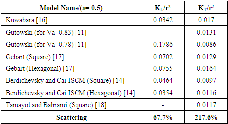
Reviewed analytical models’ calculations are compared with numerical simulations or experimental results from bibliography; but these results showed big differences between each other for the same fiber volume fraction as previously explained in the first part. This reveals the importance of performing a new numerical study simulating a real experiment and eliminating experiment’s problems.

Figure 2 shows two different fabrics which are 3D Orthogonal from 3TEX with fiber volume fraction equal to 55.76%, and a unidirectional stitched fabric (U14EU920) from SAERTEX with fiber volume fraction equal to 60.59%. Note that these real injections are done in order to affirm that the fiber arrangement is random. Thus the numerical FE modeling is performed based on a random fiber packing structure. This study measures averaged volume filling speed under a constant pressure. In other words, it is the saturated permeability value. The study is done in both longitudinal and transversal directions. A more advanced study is done for the same unit cell in a transient mode; where the flow front position is detected as function of time, taking into consideration capillary effect. Averaged unsaturated permeability is deduced. This simulation approved the consistency of static mode simulation.

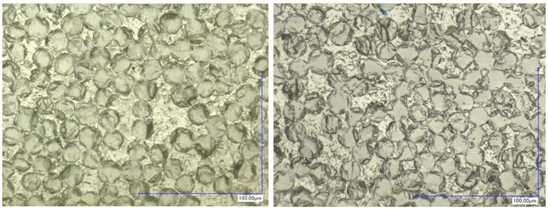Figure 2. Two fabrics: 3D Orthogonal from 3TEX at a fiber volume fraction equal to 55.76% and unidirectional stitched fabric (U14EU920) from SAERTEX at a fiber volume fraction equal to 60.59%

Values are selected from the literature at different fiber volume fractions. When two values are at the same fiber volume fraction, the permeability value which best matches with the numerical data is chosen for the comparative study. The selection between different values is convenient, taking into consideration that the unselected experiments are far from being perfect due to the inconsistency in the measuring process.

A two-level comparative study is done between all data derived from present work with the selected experiments and analytical models. From this comparison, the best models for predicting microscopic longitudinal and transversal permeability are selected.

1.4. Organization

A review of the available analytical models in the literature is established. In the second section, a numerical study is launched in order to simulate the longitudinal and transversal flow in aligned fiber beds at different fiber volume fractions in a steady state mode “saturated permeability”. In the third section, the experiments are selected based on the numerical simulations and a comparative study is launched in order to select the best analytical models based on the previous numerical simulations and selected experiments. Then, a numerical simulation in a transient free boundary problem mode is done and consequently the best analytical models will be filtered from the selection made in the third part. At the end of this study, a conclusion is deduced.

2. Analytical Models

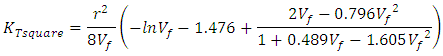
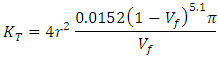
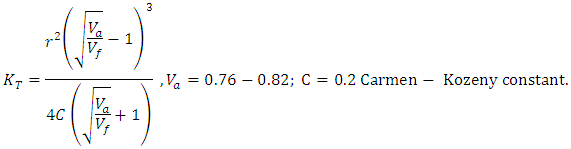
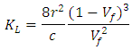
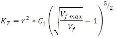
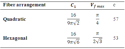
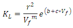
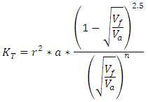
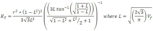
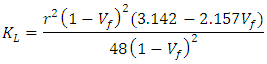
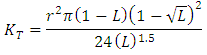
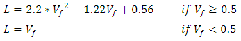
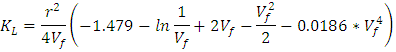
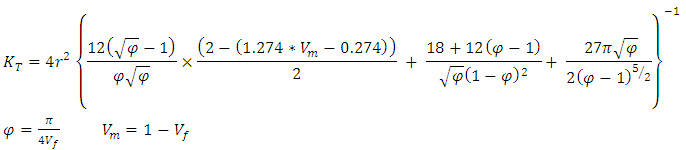
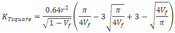
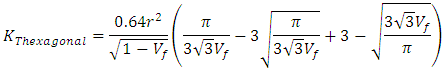
Studies on the permeability of fibrous media date back to the experimental work of Carman [28] and Sullivan [1] in 1940s, and theoretical analyses of Kuwabara [16], Happel [23] and Brenner [29]. (Appendix 1 Eq.1). Kuwabara [16], solving vorticity transport and stream function equations and employing limited boundary layer approach, predicted the permeability of flow normal to randomly arranged fibers for materials with high porosities. (Appendix 1 Eq.2,3). Happel [23] and Brenner [29] analytically solved the Stokes equation for parallel and normal flow for a single cylinder with free surface model (limited boundary layer). The boundary conditions used by Happel and Brenner [29] were different from Kuwabara’s study [16]. They hypothesized that the flow resistance of a random 3D fibrous structure is equal to one third of the parallel plus two third of the normal flow resistances of 1D array of cylinders. Later, Sangani and Acrivos [27] performed analytical and numerical studies on viscous permeability of square and staggered arrays of cylinders for the entire range of porosity values, when their axes were perpendicular to the flow direction. Their analytical models were accurate for the lower and higher limits of porosity (Appendix 1 Eq.4).

Drummond and Tahir [20] solved Stokes equations for normal and parallel flow towards different ordered structures. They used a distributed singularities method to find the flow-field in square, triangular, hexagonal, and rectangular arrays. They compared their results with numerical values of Sangani and Acrivos [27] for normal flow. The model of Drummond and Tahir [20] for predictting transversal permeability values was very close to those predicted by Sangani and Acrivos model [27], thus, it is accurate only for highly porous materials (Appendix 1 Eq.5,6,7).

Sahraoui and Kaviani [26] included inertial effects and they numerically determined the permeability of cylinders for normal flow. They also proposed a correlation which is accurate for a limited range of porosity values, i.e., 0.4 < 0.7 (Appendix 1 Eq.8).

A general mathematical model derived by Gutowski [11] assumed that the fibers make up a deformable, nonlinear elastic network. The resin flow is modeled using Darcy’s Law for anisotropic porous medium. (Appendix 1 Eq.9). Gebart [17] derived an analytical model to predict the unidirectional permeability starting from Navier-Stokes equation. (Appendix 1 Eq.10, 11) In 1993, Berdichevsky and Cai [14], after performing some numerical simulations, considered that the permeability depends on the fiber volume fraction and the ultimate fiber volume fraction. Then they derived a unified empirical model. (Appendix 1 Eq.12, 13). Then in the same year, they developed their model “self consistent method model” to “improved self consistent model “[14], where Stokes flow and Darcy flow are then respectively considered at different regions. Boundary and interface conditions as well as two consistency conditions including the total amount of the flow and the energy dissipation, are applied accordingly. The permeability is solved based on these considerations. This improved permeability model captures the flow characteristics in a given fiber bundle. In the transverse flow case, the gaps between neighboring fibers govern the flow resistance. The derived expression for the transverse permeability contains two variables, the averaged fiber volume fraction and the maximum packing efficiency, which adequately describe the status of a fiber bundle. (Appendix 1 Eq.14,15).

Phelan and Wise [25] studied the transverse flow through rectangular arrays of porous elliptical cylinders and derived a semi-analytical model based on lubrication theory. The Brinkman equation is used to model the flow inside porous structures, and the Stokes equation to model the flow in the open media between the structures (Appendix 1 Eq.16). Lee and yang [6] considered the flow as a non-Darcy flow through a porous medium. The continuity equation and the momentum equation in pore scale are solved on a Cartesian grid system. To avoid the numerical difficulties resulting from the flow domain of irregular shape, the weighting function scheme along with the APPLE algorithm and the SIS solver are employed. The Darcy-Forchheimer drag (pressure drag) is then determined from the resulting volumetric flow rate under a prescribed pressure drop to derive their permeability model. (Appendix 1 Eq.17). Brushke and Advani [22] considered the flow across regular arrays of cylinders. The analytic solutions are matched to produce a closed form solution. This is done by employing the lubrication approach for low porosities and the analytic cell model solution for high porosities. (Appendix 1 Eq.18). Using numerical simulations, Van der Westhuizen and Du Plessis [24] proposed a correlation for the normal permeability of 1D fibers. (Appendix 1 Eq.19,20). Tamayol and Bahrami [21] performed studies on the ordered fibrous media towards normal and parallel flow, thus the permeability is obtained analytically. To predict permeability, a compact relationship is suggested by modeling 1D touching fibers as a combination of channel-like conduits. Moreover, analytical relationships are developed for pressure drop and permeability of rectangular arrangements. This is performed by using an “integral technique” and simulating a parabolic velocity profile within the unit cells. The experimental results collected by others for square arrangement confirm the data of the developed models. (Appendix 1 Eq.21,22).

Tamayol and Bahrami [18] studied the transverse permeability of fibrous porous media both experimentally and theoretically. A scale analysis technique is used in order to obtain the transverse permeability of fibrous media with a variety of fibrous matrices including square, staggered, and hexagonal unidirectional fiber arrangements. In this field, a relation is designated between the permeability and the porosity, fiber diameter, and tortuosity of the medium. Also, the pressure drop in several samples of tube banks of different arrangements and metal foams is measured in the creeping flow regime. The obtained results are then utilized to calculate the permeability of the samples. The developed compact relationships are confirmed by performing comparison with the present experimental results and the data given by others. (Appendix 1 Eq.23,24).

The models listed in this section predict the longitudinal and transversal microscopic permeability “K_L” and “K_T”, for most models the permeability is a function of the fiber radius “r” and the fiber volume fraction “V_f”. However, for some models the permeability is linked to other parameters like the maximum fiber packing factor “V_fmax”, geometrical effects “C, C₁…’’, packing structure (hexagonal or square or other structures) “V_a”.

3. Numerical Steady State Method and Results (Saturated Permeability)

In this section, a FE modeling, using COMSOL MULTIPHYSICS software which consists of a CFD analysis is performed to estimate the microscopic saturated permeability value of multiple cases involving porous media. Two cases were studied, which involve a longitudinal and a transversal flow through certain porous media in order to predict the saturated permeability value of the media. A finite element (FE) based model for viscous, incompressible flow through random packing of fibers is employed for predicting the permeability associated in the porous media.

3.1. Methodology

In this study, random arrangement of fiber is considered, which is shown to be as most representative for a real fiber stacking. Figure 3 shows the 2D unit cell dimensions for transverse permeability predictions having a length of 0.33mm and a width of 0.1mm. However, the 3D unit cell dimensions for longitudinal permeability are length = 0.33mm, width = 0.1mm, and depth=1mm. Different fiber contents are selected to cover a wide range of porosities (0.3 to 0.9) for both transversal and longitudinal simulations Figure 4 and Figure 5. Porosities are selected with respect to available data from the bibliography; refer to the introduction.

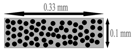Figure 3. Unit cell Dimensions

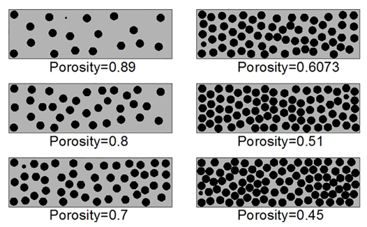Figure 4. Selected porosities for transversal flow simulation

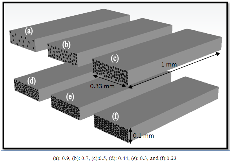Figure 5. Selected porosities for transversal flow simulation

The model used is based on Navier-Stokes equation, where the fluid is subjected to the action of a body force F, the Navier-Stokes equation can be written as follow in equation (2).

(2)

Where ρ is the density, v is the velocity of the fluid, t is time, P is the pressure, and F is the volumetric force. Permeability in fluid mechanics is a measure of the ability of a porous material to allow fluid to pass through it. The most widely used equation for describing flow is Darcy’s equation for flow through porous media. Fluids modeled by Darcy’s law must obey the assumptions used to formulate the Navier Stokes equation. Namely, fluids must have a constant density and viscosity and must obey Newtonian behavior [30].

(3)

μ is the viscosity of the fluid, is the pressure drop, K is the permeability tensor of the porous medium, is the velocity of the fluid, and H is the depth of the unit cell.

The flow Reynolds number should be kept sufficiently low to ensure negligible effects of inertial terms. Reynolds number equation (4) is ranged between 1 and 10 (1< Re < 10) [31], Where is the equivalent pore diameter.

(4)

The porosity of a porous medium is the ratio of the pore volume to the total volume of a representative sample of the medium; it can be calculated using this equation (5).

(5)

Where N is the number of fibers, d is the fiber diameter and is the total surface of the unit cell. So for a selected fluid “selected viscosity”, on a selected porosity and on a predefined inlet and outlet pressures the filling time is obtained from the simulation. Using equation (3) the saturated permeability is calculated.

3.1.1. Selected Porosities

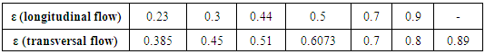
Based on the available data from literature, different porosities were selected Table 6, in order to predict the microscopic permeability values on these porosities.

Table 6. Porosity values for performing the study

3.1.2. Flow Type and Fluid Properties

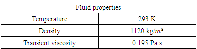
In fluid transients, laminar flow occurs when a fluid flows in parallel layers, with no disruption between the layers. At low velocities, the fluid tends to flow without lateral mixing, and adjacent layers slide past one another like playing cards. Neither cross-currents perpendicular to the direction of flow, nor eddies or swirls of fluid exist. In laminar flow, the motion of the particles of the fluid is very orderly with all particles moving in straight lines parallel to the walls. The fluid used in simulations is epoxy resin which has the properties shown in Table 7.

Table 7. Fluid properties of epoxy resin

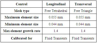
3.1.3. Meshing Technique

CFD simulation requires that the computational domain gets divided into small cells where the flow is modeled and the flow equations are solved. COMSOL MULTIPHYSICS software is used to generate the mesh that will be used in simulations involving random form. The generated mesh for longitudinal and transversal unit cells and meshing controls are shown respectively in Figure 6 and Table 8. For example for a longitudinal permeability unit cell for a V_f of 0.5, the complete mesh consists of 1603619 domain elements, 461336 boundary elements, and 57153 edge elements.

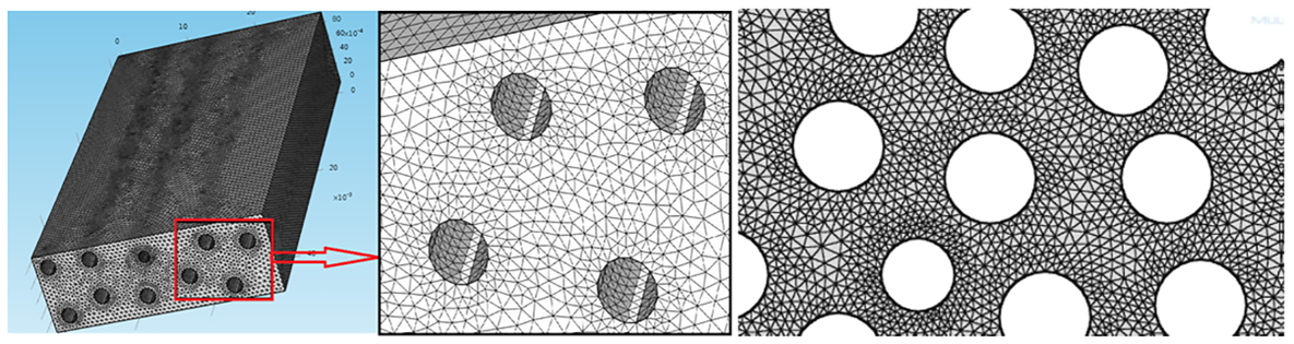Figure 6. Generated mesh for longitudinal and transversal unit cells

Table 8. Meshing Conditions

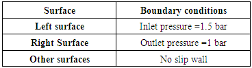
3.1.4. Boundary Conditions

After the mesh process is completed, the next step is to specify the boundary conditions. Similar boundary conditions were used in all the simulations, which are shown in Table 9. Type of boundary condition: constant pressure with no viscous stress.

Table 9. Boundary Conditions

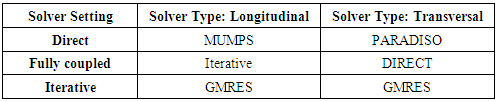
3.1.5. Solver Settings

Since the flow in the simulations that were performed is supposed to be Laminar (low velocity flow), the Laminar model that solves the Navier-Stokes equations was used Table 10.

Table 10. Solver Settings for stationary solver

Where MUMPS: Multifrontal Massively Parallel Sparse (direct Solver), GMRES: Generalized Minimum Residual (iterative method).

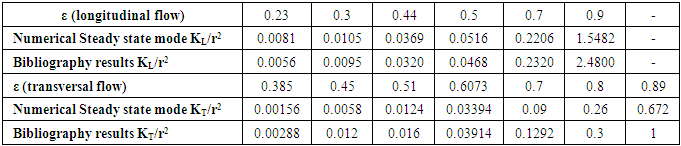
3.2. Results and Comparison for Numerical Simulations in Steady State Mode

The results of the calculated permeability values are shown in the Table 11. In the next section, two comparative studies are launched for both longitudinal and transversal microscopic permeability values; where in the results derived from numerical steady state mode simulations and experimental measured results will be compared with results derived from available analytical models.

Table 11. Permeability results of the numerical simulation in steady state mode for longitudinal and transversal flow with the selected measurements

A comparison is launched between analytical models on one hand and the bibliography results and numerical results on the other hand. This comparison aims to choose the analytical models which best matches with these results.

3.2.1. Comparison for Longitudinal Flow (Steady State mode)

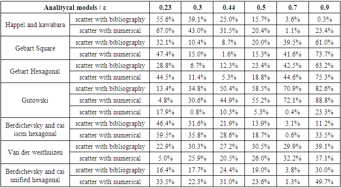
As shown in Table 12 and Chart 1, Gutowski model values compared with the bibliography results show big scatter at most of the selected porosities such as 34.8% at porosity ε = 0.3, and keeps rising till 70.9% at porosity ε = 0.7. Similarly, the comparison of these models’ values with the simulation reveals almost same scattering ranging between 30.6% and 72.1%.

Table 12. Scattering values derived from the comparison with the bibliography results and numerical simulation results

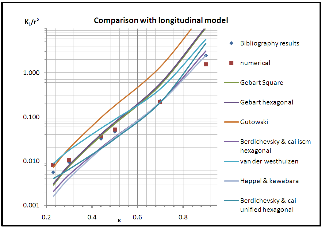Chart 1. Comparison between longitudinal models

Van der Westhuizen model results reveal large scattering when compared to bibliography and numerical results. This scatter starts from 22.9% and rises up till 39.1%. Gebart (square and hexagonal) models' results exhibit low scattering only on the porosities 0.3 and 0.44 such as 6.7% and 8.7% with the bibliography results, and 1.6% and 5.3% when compared with the numerical ones. But the scattering increases sharply at porosities less or greater than 0.3 and 0.44, ranging between 23.4% and 47.4% when compared to bibliography and numerical results. Analogously, the models Berdichevsky and Cai ISCM (hexagonal), Berdichevsky and Cai unified (hexagonal), and Happel and Kuwabara show an intersection with the bibliography and numerical results at a single porosity which is 0.7 (scatter around 3% and 1% when compared with the bibliography and numerical results respectively), while it seems to be high on the other porosities for the entire three models. The models Gutowski, Van der Westhuizen, Gebart (square and hexagonal), Happel and Kuwabara, Berdichevsky and Cai ISCM (hexagonal), and Berdichevsky and Cai unified (hexagonal) are excluded due to the big scatter between the results of these models when compared to the bibliography and numerical values on almost all of the selected porosities.

On the other side of the coin by referring to Table 13 and Chart 2, it is obviously realized that there are four models that give values which are very close to the bibliography and numerical values, evidenced by the low scattering between the values at most of the selected porosities. One of these models is Tamayol and Bahrami which when compared with bibliography values has a range of scatter lying between 0.3% at porosity ε = 0.7, and 7.1% at porosity ε = 0.44. And compared to the numerical results, it also shows very low scattering, as shown in the table; 1.9% at porosity 0.3 and 7.9% at porosity 0.5. Drummond and Tahir is also one of the models that have results close to the bibliography and numerical results. Examples are 3.4% scatter with the bibliography result at porosity 0.44 and 3.3% scatter with numerical value at porosity 0.7. But the scatter is relatively high (25.3%) compared to the bibliography result on porosity 0.23.

Table 13. Scattering results derived from the comparison with the bibliography results and numerical simulation results

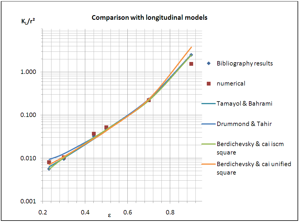Chart 2. Comparison between longitudinal models

The other two models which show very low scatter in comparison with the bibliography and numerical results are Berdichevsky and Cai ISCM square and Berdichevsky and Cai unified square. The scattering with the bibliography results ranges between 0.4% and 4.0% for the first model and between 0.7% and 11.3% for the second one. Similarly, the comparison with the numerical study results also reveals very low ranges of scattering, being between 0.4% and 17.9% for the first model and between 2.1% and 13.7% for the second.

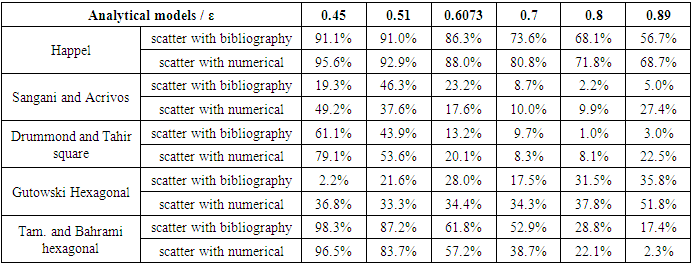
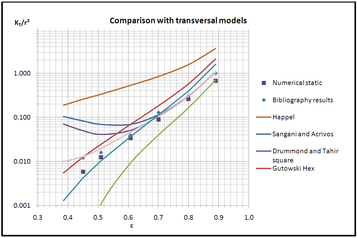
3.2.2. Comparison for Transversal Flow (Steady State Mode)

By referring to Table 14 and Chart 3, Happel shows very high scattering with bibliography results on all selected porosities, with the least scattering equal to 56.7% at porosity 0.89 and greatest one equal to 91.1% at porosity 0.45. The scattering is similarly high with numerical results ranging between 68.7% and 95.6%.Gutowski (hexagonal) reveals distinct scattering values but the overwhelming majority lies between 21.6% and 51.8%.Tamayol and Bahrami (hexagonal) displays great scattering values with the bibliography results on one hand and with the numerical results on the other hand, which range between 17.4% and 98.3%. The models having great scatter with the bibliography and numerical results are excluded from the study. Those are Happel, Gutowski (hexagonal), and Tamayol and Bahrami (hexagonal) models. Both models Sangani and Acrivos and Drummond and Tahir (square) when compared with both bibliography and numerical results show big scattering at lower porosities and smaller scattering values at higher porosities, which reveals the ineffectiveness of these models in our study. The comparison of Sangani and Acrivos results with the bibliography results show scattering values 8.7%, 2.2% and 5.0% at porosities 0.7, 0.8, and 0.89 respectively; while the scattering is high at lower porosities (19.3%, 46.3%, 23.2%). Similarly, when compared to the numerical results, the scattering values are divided into two halves, some are high and the others are relatively low. Drummond and Tahir scattering values with numerical and bibliography values are mostly greater than 20% at the first three porosities, and lower than 20% at the next three ones.

Table 14. Scattering results derived from the comparison with the bibliography results and the numerical simulation results

Chart 3. Comparison between transversal models

As shown in the Table 15 and Chart 4, Bruschke and Advani model shows mostly scattering values greater than 15%. For example, compared with bibliography values, some of the scattering values are 13.6%, 15.5%, and 24.5%. And the comparison with the numerical results shows scattering values 29.8% at porosity 0.45, 23.0% at porosity 0.51, 22.4% at porosity 0.8. Gebart (square), Gutowski (square), and Van Der Westhuizen intersect with the bibliography and numerical results at a single porosity each. That's to say, Gebart (square) showed low scattering with both bibliography and numerical values (4.5% and 8.2%) at porosity 0.51, but the scattering is higher at the entire other porosities. Similarly, Gutowski has a single intersection with the bibliography and numerical results, and that's at porosity 0.6073 with scattering 3.1% compared to bibliography result and 4.0% compared to numerical result, while the scatter increases at the other porosities. In addition, Van Der Westhuizen values intersect with the bibliography and numerical results at porosity 0.8 and the other scattering values take place between 2.9% and 26.5%. Bruschke and Advani, Gebart (square), and Gutowski (square) are the most likely to be eliminated from the study.

Table 15. Scattering results derived from the comparison with the bibliography results and numerical simulation results

Chart 4. Comparison between transversal models

The models Drummond and Tahir (hexagonal), Sahraoui and Kaviany, Berdichevsky and Cai ISCM (square), Phelan and Wise, Lee and Yang, Berdichevsky and Cai unified Model Square, and Berdichevsky and Cai unified model Hex exhibit in most of the comparisons with both bibliography and numerical results scattering values less than 15%.

Each one of the models mentioned in the Table 16 and Chart 5 shows results which have very low scattering when compared with the bibliography and numerical results, which is in most of the cases less than 15%. All models having a scattering less than 15% are selected to be discussed in the next section.

Table 16. Scattering results derived from the comparison with the bibliography results and numerical simulation results

Chart 5. Comparison with transversal models

4. Numerical Simulation in a Transient Free Boundary Problem Mode

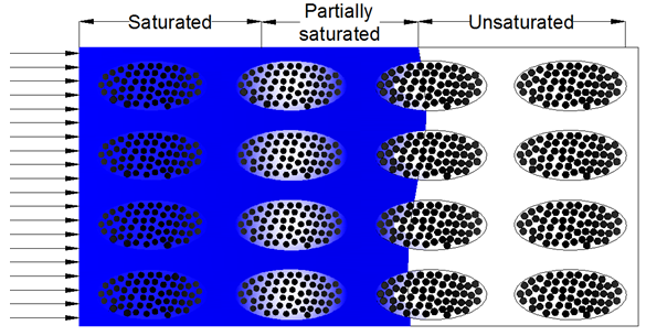
In the previous section the transversal numerical simulation was performed in a steady state mode in which a single phase problem was solved, where the studied fluid is located in the saturated region Figure 7. The capillary pressure and surface tension were neglected; thus the measured microscopic permeability value was the transversal saturated microscopic permeability.

Figure 7. Flow front progression

In this part, a numerical simulation in a transient mode is done; where capillary pressure and surface tension are taken into account. The flow front progression is registered in function of time, and corresponding velocity values for selected flow front positions are recorded. Average permeability is then derived from local permeability values. Due to computational limitations, only the transversal microscopic unsaturated permeability will be predicted. The selected models from the previous comparative study between the numerical results (steady state mode), analytical models, and bibliography measurements will be compared with results derived from the new simulations (transient mode).

4.1. Simulation Parameters in Transient Mode

The two fluids selected in this simulation are: Air and Epoxy Resin. Same meshing technique and boundary conditions are used when simulating in a transient mode, whereas, different parameters are took into consideration when the transient simulation is performed, which are the surface tension, mobility, and relative tolerance.

4.1.1. Surface Tension

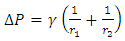
The COMSOL MULTIPHYSICS allows the calculation of capillary pressure between each two fibers. Capillary pressure is the necessary pressure to force “non-wetting fluid” to displace the “wetting fluid” in a capillary. Capillary pressure [32] can be mathematically expressed as P_c, equation (6); where P_nw and P_w are the pressures of the non-wetting phase and wetting phase across the interface

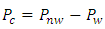(6)

In other words, capillary pressure is defined by the capillary forces divided by the surface between the two fibers or between the fiber and the plane. Young-Laplace equation [33] Eq 7 is of fundamental importance in order to understand the capillary forces; where r1 and r2 are two principal radii of curvature, γ is the surface tension between air and fluid Figure 8 for Epoxy Resin (γ=44*10^-3 N/m), σ_SA is the surface tension between the solid and air, σ_SW is the surface tension between solid and fluid and Ψ is the wetting angle.

(7)

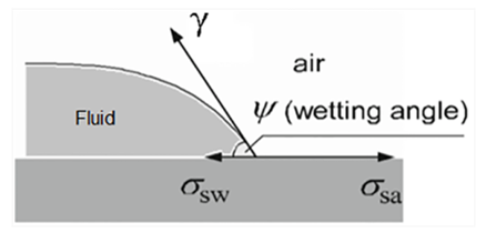Figure 8. Wetting angle between fluid and surface

Figure 9 and Table 17 show the capillary forces in sphere-sphere & sphere-plane geometries, where D is the distance between two interacting solid surfaces, F is the capillary force, l is the Azimuthal radius of a meniscus, R₁ and R₂ are the radii of two spherical particles, r is the meridional radius, β is the angle characterizing position of three phase contact line on sphere, γ is the surface or interfacial tension and θ1, θ2 contact angles on the two interacting surfaces.

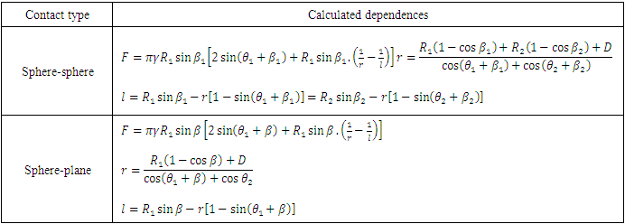
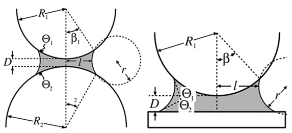Figure 9. Fluid subjected to capillary forces in sphere-sphere or sphere-plane geometries [33]

Table 17 [33]

4.1.2. Mobility and Relative Tolerance

The mobility is related to the time-scale of the Cahn-Hiliard diffusion and therefore governs the diffusion-related time scale of the interface. The χ parameter should be optimized to maintain a constant interface thickness and avoid damping the convective motion. A very high mobility can also lead to excessive diffusion of droplets [34]. Relative tolerance is the permitted variation in some measures and characteristics of an object or work piece. It indicates the precision of reading flow time results.

4.2. Results for Transient Simulation

The flow front position is recorded at different selected filling time intervals, after extracting the set of results of filling time and correspondent flow front position. The elementary permeability is calculated using Darcy’s law. Then the total permeability is calculated by interpolating these results. Figure 10 shows the flow front observed at two different positions. The local permeability values at successive positions are calculated based on equation (3); then an average permeability value is calculated using equation (8).

(8)

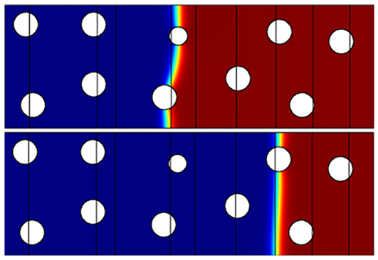Figure 10. Flow front observed at two different positions for 0.89 porosity unit cell

The following Table 18 shows the results of the simulation in a transient mode which gives rise to unsaturated microscopic permeability values.

Table 18. Results of the numerical simulation in transient mode

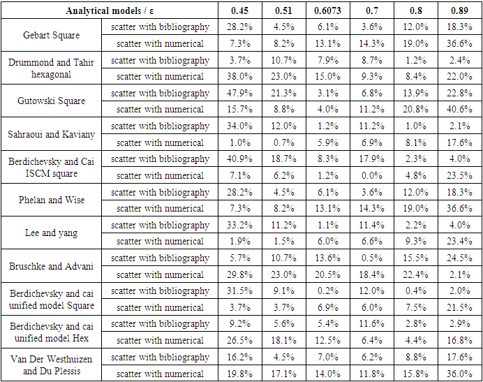
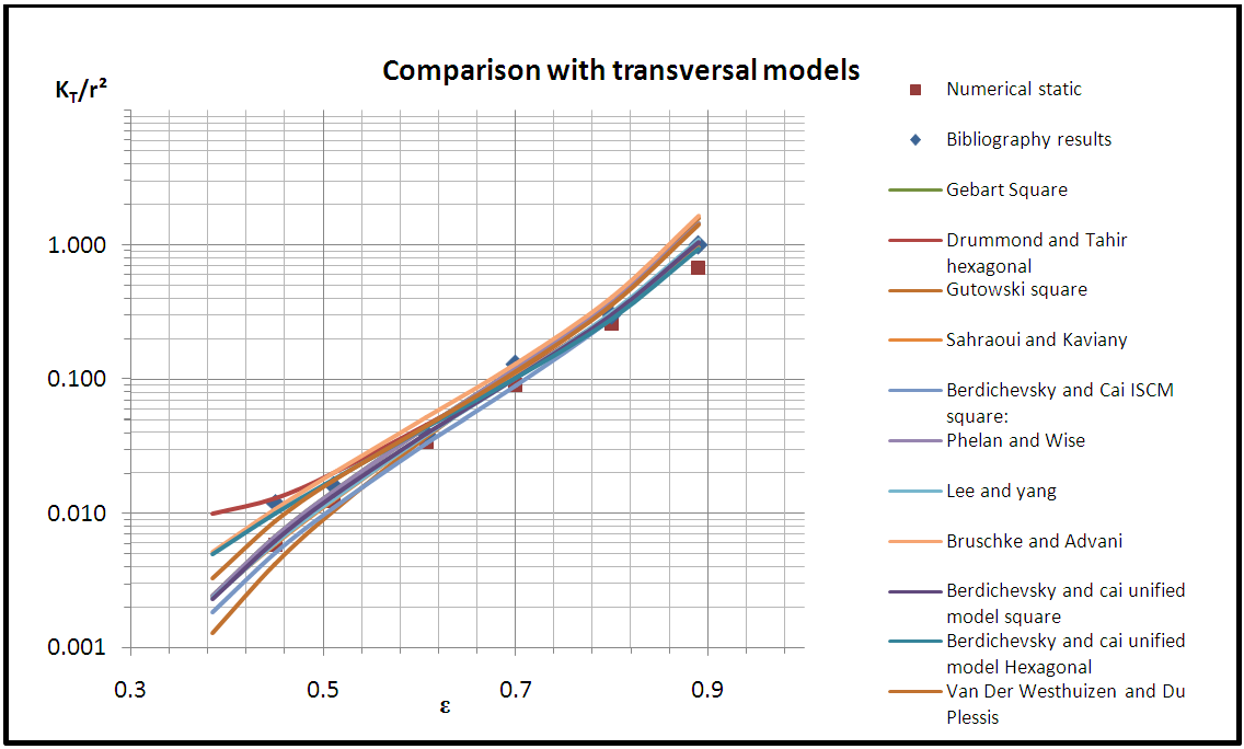
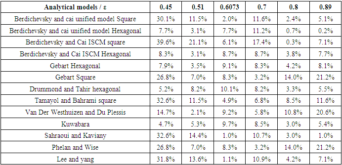
4.3. Comparative Study (Transient Mode)

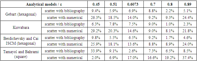
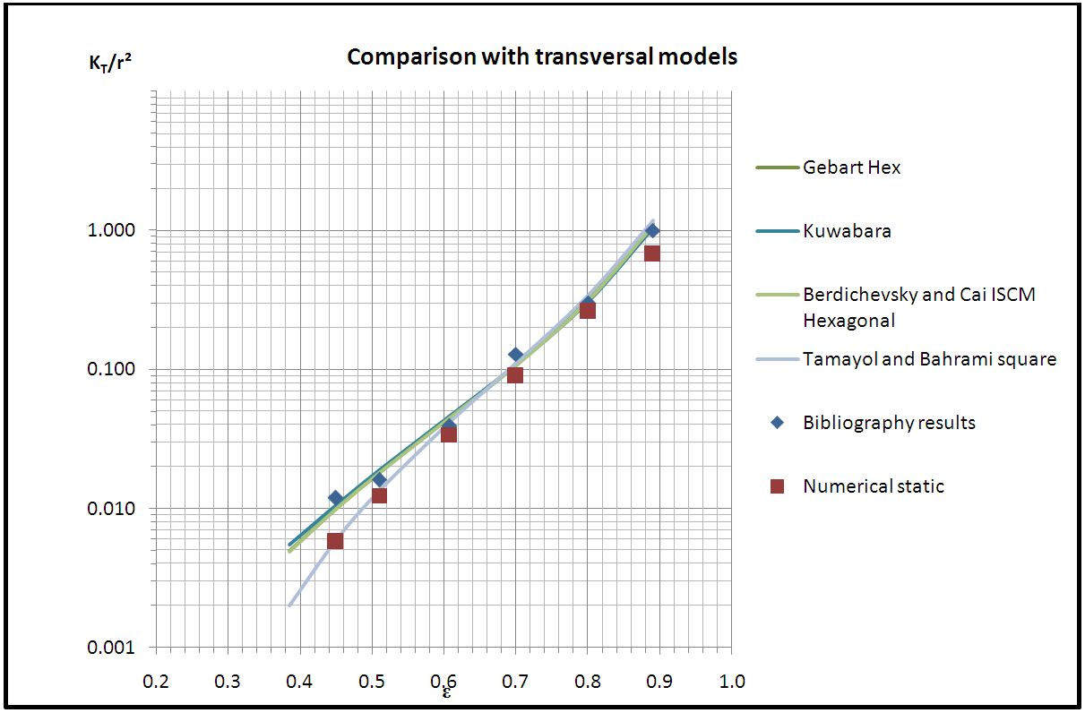
The models previously selected from the comparative study with steady state mode numerical simulation are subjected to sorting, in which the models with relatively lowest scattering in comparison with numerical simulation in transient mode are considered to be the most suitable for obtaining the transversal microscopic permeability. In this comparative study the chosen models are those having a scattering less than 10%.

Table 19 indicates that Berdichevsky and Cai unified model (square) shows three scattering values 2%, 2.4%, and 5.1% which are less than 10%, at porosities 0.6073, 0.8, and 0.89 respectively. On the other hand, the other three values are greater than 10% (30.10% at porosity 0.45, 11.20% at porosity 0.51, and 11.60% at porosity 0.7).

Similarly, Berdichevsky and Cai ISCM square, Gebart Square, Tamayol and Bahrami square, Van Der Westhuizen and Du Plessis, Sahraoui and Kaviany, Phelan and Wise, and Lee and yang exhibit in each one of them three values of scattering less than 10% and other three values greater than 10%.

Whereas, Berdichevsky and Cai ISCM hexagonal, Gebart hexagonal, Drummond and Tahir hexagonal, and Kuwabara are better relatively, due to the scattering values that are less than 10% at all selected porosities as shown in Table 19.

Table 19. Scattering derived from the comparison with the numerical simulation in transient mode results

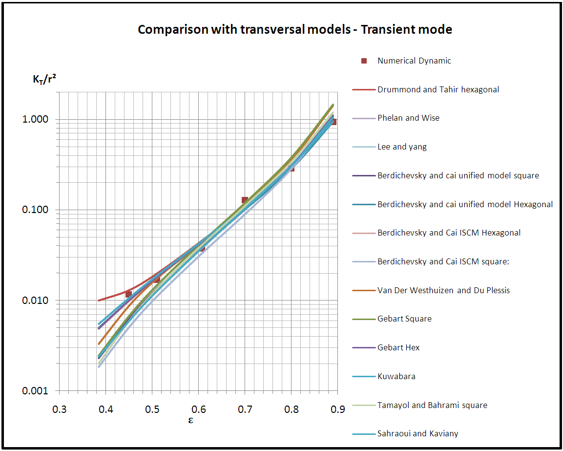Chart 6. Comparison with transversal results

5. Discussion and Analysis

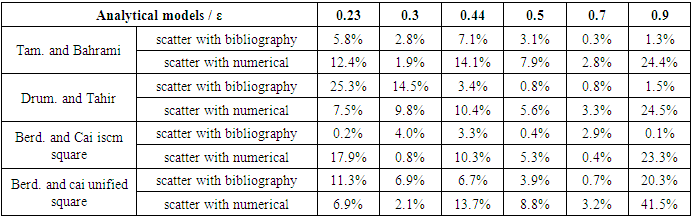
The comparative studies listed in the previous part of the article are done in order to choose the best models which serve in predicting the microscopic permeability.

After performing the comparison between the longitudinal models and the results of the bibliography and numerical simulations in steady state mode, the models Bahrami and Tamayol, Drummond and Tahir, Berdichevsky and Cai ISCM square, and Berdichevsky and Cai unified square are elected to be the most accurate in predicting longitudinal microscopic permeability. This selection was done based on the low scattering values in these comparisons.

Regarding the comparative study between the transversal models and the results of the bibliography and numerical simulations in steady state mode, a primary selection was done which highlighted the models that show lower scattering values in comparison with the other models. The selected models are Berdichevsky and Cai unified model Square, Berdichevsky and Cai unified model Hexagonal, Berdichevsky and Cai ISCM Square, Berdichevsky and Cai ISCM Hexagonal, Gebart Hexagonal, Gebart Square, Drummond and Tahir Hexagonal, Tamayol and Bahrami Square, Van Der Westhuizen and Du Plessis, Kuwabara, Sahraoui and Kaviany, Phelan and Wise, and Lee and Yang.

Those models are subjected to a secondary selection process which aims to ensure choosing the most convenient models able to fulfill the prediction of transversal microscopic permeability when recommended in any study. This selection process is spread on two steps. First, a numerical simulation in transient mode is done at the same given unit cells previously. This simulation solves a dual phase problem and thus gives permeability value which is more realistic and resembling a real experiment. Second, a comparative study is done between the analytical results of the models and the obtained results from the numerical simulation in transient mode. The models which show the least scattering in this comparison are Berdichevsky and Cai ISCM (hexagonal), Gebart (hexagonal), Drummond and Tahir (hexagonal), and Kuwabara. These selections are the most convenient models for predicting transversal microscopic permeability which is involved in obtaining the permeability tensor value.

6. Conclusions

The microscopic permeability analytical models were subjected to sorting by comparing their permeability outputs to results derived from other prediction methods. A numerical study was performed, distinguished by utilizing a unit cell with random fiber arrangement which was most representative for real experiment. A comparative study was done between analytical modeling, bibliography, and numerical results. Its analysis presents that Bahrami and Tamayol, Drummond and Tahir, Berdichevsky and Cai ISCM and unified (square) models have good agreement with this data for longitudinal microscopic permeability components. Concerning transverse microscopic permeability, Berdichevsky and Cai ISCM (hexagonal), Gebart (hexagonal), Drummond and Tahir (hexagonal), and Kuwabara models were elected to be the most accurate models. On the other hand, transient mode simulations gave rise to results synchronized with the static mode simulations, which revealed the consistency of the study.

The profit of this study is to know the most convenient analytical models to predict the microscopic permeability in unidirectional fiber bundles. Furthermore, in order to calculate an accurate permeability tensor, the value of the microscopic permeability should be obtained precisely. Moreover, the microscopic permeability could be employed in some other studies such as capillary pressure or permeability modeling studies.

Nomenclature

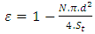
K_L: Longitudinal microscopic permeability

K_T: Transversal microscopic permeability

ε: Resin volume fraction

V_f: Fiber volume fraction

V_a: Maximum fiber volume packing factor

Appendix

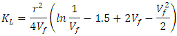
(Eq.1)

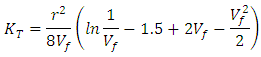
(Eq.2)

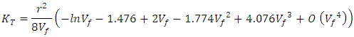
(Eq.3)

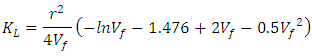
(Eq.4)

(Eq.5)

(Eq.6)

(Eq.7)

(Eq.8)

(Eq.9)

(Eq.10)

(Eq.11)

(Eq.12)

(Eq.13)

Where

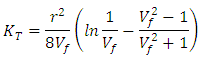
(Eq.14)

(Eq.15)

(Eq.16)

(Eq.17)

(Eq.18)

(Eq.19)

(Eq.20)

(Eq.21)

(Eq.22)

(Eq.23)

(Eq.24)