Sandeep Medikonda1, Ala Tabiei1, Rich Hamm2
1Department of Mechanical and Materials Engineering, University of Cincinnati, Cincinnati, OH, USA
2P&G, Cincinnati, OH, USA
Correspondence to: Sandeep Medikonda, Department of Mechanical and Materials Engineering, University of Cincinnati, Cincinnati, OH, USA.
| Email: |  |
Copyright © 2017 Scientific & Academic Publishing. All Rights Reserved.
This work is licensed under the Creative Commons Attribution International License (CC BY).
http://creativecommons.org/licenses/by/4.0/

Abstract
A micromechanical model based on the physically viable sub-cell boundary conditions is developed and implemented for use with uni-directional composite laminates in the explicit finite element method. Stress-strain relations have been presented in a three-dimensional context and hence can be used with solid elements. The objective of this work is to study the effect of boundary conditions in accurately estimating the elastic properties of a uni-directional composite lamina. In order to achieve this, the developed micro-model has been studied alongside 2 other models with different boundary conditions specified in the literature. Numerical results are generated for engineering constants by the considered models and compared against each other for different laminas. In particular, transverse and shear modulus have been analyzed in detail alongside popular analytical methods and verified against available experimental results for various volume fractions. Good agreements have been observed for the presented model in comparison with the experimental results.
Keywords:
Unidirectional Composites, Micro-mechanical model, Representative Volume Cell (RVC), Iso-stress boundary conditions, Iso-strain boundary conditions, Elastic constants
Cite this paper: Sandeep Medikonda, Ala Tabiei, Rich Hamm, A Comparative study on the Effect of Representative Volume Cell (RVC) Boundary Conditions on the Elastic Properties of a Micromechanics Based Unidirectional Composite Material Model, International Journal of Composite Materials, Vol. 7 No. 2, 2017, pp. 51-71. doi: 10.5923/j.cmaterials.20170702.03.
1. Introduction
Composite materials have a wide range of applications, their use as structural components in automobiles, air and space vehicles is an attractive option because of their high impact tolerance, high stiffness-to-weight and strength-to-weight ratios. As a consequence, over the last decade, an increased usage of composite materials has been observed. The constitutive relations used to numerically model composite materials can be characterized into two groups, macro-mechanical models and micro-mechanical models. Micro-mechanical models provide the overall behavior of the composite from the properties of the individual constituents (e.g. fibers and matrix) and their interactions. Macro-mechanical models, on the contrary, replace the heterogeneous structure of the composite with a homogeneous medium consisting of anisotropic properties (which need to be determined). While, macro-mechanical material models require less computational work, they fall short in accurately capturing composite response especially for complex load histories. On the other hand, micro-mechanical material models despite requiring more computational work can overcome these short comings. Sophistications in computing technology have made it feasible to implement the micro-mechanical models alongside non-linear finite element (FE) codes. The popular transient non-linear FE code LS-DYNA [1] has been chosen in the current work as it offers a very simple interface to implement user material models. Micromechanical analyses can be further divided into mechanics of materials (MoM) and theory of elasticity (ToE) approaches. While the MoM approach is based on simplifying assumptions regarding the hypothesized behavior of the composite, the ToE apporach is characterized by getting rid of some of these assumptions and more rigorously satisfying the equilibrium, continuity and compatibility conditions. Because the focus of this paper is on the implementation of the model in a finite element framework, it needs to be a reasonable mix of simplicity and accuracy; hence the mechanics of materials approach was used.In the explicit solution scheme of the finite element analysis, the accelerations are solved for as the inverse of the diagonal mass matrix times the force vector. Once accelerations are known at time ‘n’, velocities are calculated at time ‘n+1/2’, and displacements at time ‘n+1’. This displacement increment causes an increment of strain at a material point. The strain is passed into the material model to calculate the incremental stress. Stiffness, strains, and stresses are tracked at the material points within each element. This information is provided by the micromechanical composite material model, which interfaces with the nonlinear explicit finite element code. The heterogeneous nature of the composite material is hidden from the main analysis code. Micromechanical theory discussed in this work predicts the average behavior of the lamina as a function of the constituent properties and the local boundary conditions; this is an important advantage as no prior knowledge of the lamina response is required.In one of the earliest attempts at including micro-mechanics into the FE analysis of composite structures, Adams and Crane [2] developed a micro-mechanical model using the representative volume element. However, this model has been observed to computationally expensive. Pecknold and Rahman [3] proposed a simpler micro-model which has been a basis for the current study. A significant advantage of the Pecknold and Rahman model is its capability to analyze elastic as well as in-elastic constituents (e.g. visco-elastic and visco-plastic), thus forming a unified approach in predicting the overall behavior of the composite material.The objectives of the current work are:1. Use physically viable sub-cell boundary conditions and modify the Pecknold and Rahman micro-model. Subsequently, derive constitutive relations for the RVC based on these modified boundary conditions. 2. Implement this material model as a user subroutine in LS-DYNA and compare the elastic properties predicted against similar numerical models (same RVC but different boundary conditions), analytical models and experimental results presented in the literature for various laminae.
2. Geometric Description of the Micro-mechanical Model
A schematic of the representative volume cell (RVC) used to develop the micro-mechanical relations is shown in Figure. 1. The basic structure of the RVC which was originally proposed by Pecknold and Rahman [3] has been used by Tabiei et al. [4-6] in several studies to accurately capture different behaviors of uni-directional composites.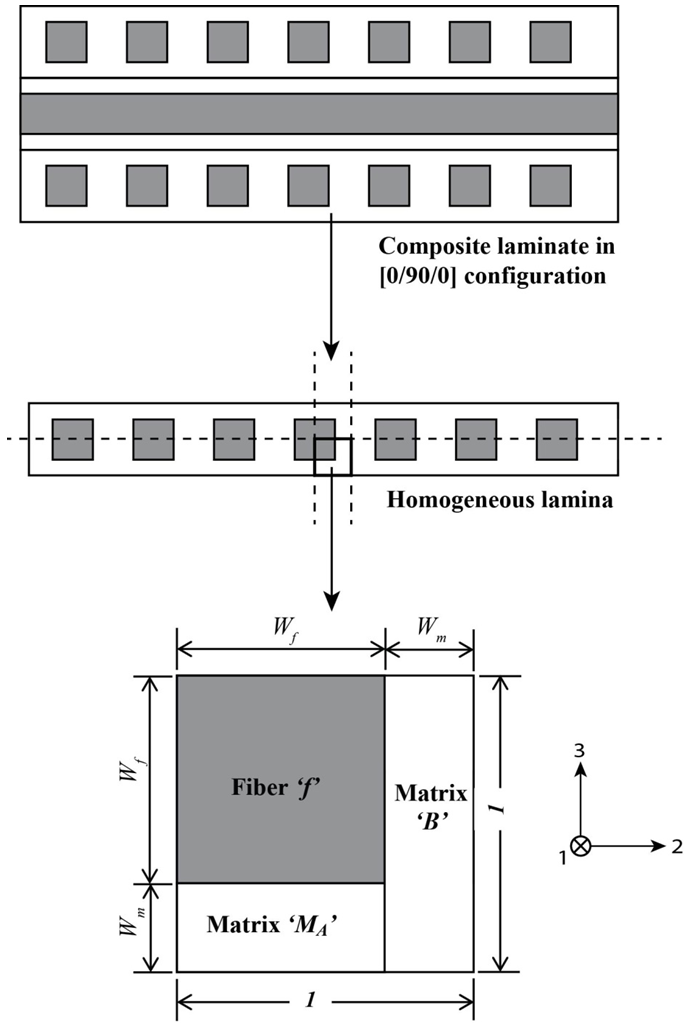 | Figure 1. Modeling strategy and representative volume cell of the unidirectional composite |
The underlining premise of the micro-model is based on the assumption that the internal micro-structure of the lamina consists of periodic square fibers. In addition, the following assumptions are made regarding behavior of the constituents and the composite as a whole:1. The fiber material is homogeneous and linearly elastic.2. The matrix material is homogeneous and linearly elastic.3. The fibers are positioned in the matrix such that the composite lamina is a homogenous material with linearly elastic behavior.4. There is a complete and strong bond at the interface of the constituent materials.The unit cell is divided into three sub-cells: one fiber sub-cell, denoted as f, and two matrix sub-cells, denoted as MA and B respectively. The three sub-cells are grouped into two parts: material part A consists of the fiber sub-cell f and the matrix sub-cell MA, and material part B consists of the remaining matrix B. The dimensions of the unit cell are 1 × 1 unit square. The dimensions of the fiber and matrix sub-cells are denoted by Wf and Wm.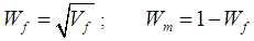 | (1) |
where Vf is the fiber volume fraction. As explained in a later section, effective stresses in the RVC are determined from the sub-cell values in two phases: first, stresses in fiber f and matrix MA are combined to obtain effective stresses in part A which are then combined with stresses in matrix B to obtain the effective RVC stresses.
3. Boundary Conditions of the Micro-mechanical Model
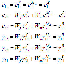
Once the finite element solver passes the average strains of the RVC into the user material model sub-routine, micromechanical relations are used to obtain the average stresses using Parallel (Iso-strain) – Series (Iso-stress) assumptions. The RVC is divided into three sub-cells and sub-cells are either in parallel or in series for the various components of strains and stresses.If two sub-cells are in parallel for a particular directional component, then the corresponding strains are equal and the average RVC stress in that direction is given by the rule of mixture applied on the average stresses in those sub-cells. On the other hand, if two sub-cells are in series for a particular component, then the corresponding stresses are equal and the average RVC strain in that direction is given by the rule of mixture applied on the strains in those sub-cells.One of the distinguishing aspects of the current work as compared to the micro-model presented by Pecknold and Rahman [3] and subsequently used by Tabiei et al. [4-6] is the manner in which iso-stress and iso-strain boundary conditions have been applied on individual components. In order to simplify the complexity of the micro-mechanical relations, Tabiei and Babu [6] have used the iso-strain boundary conditions in both phases of homogenization. Whereas, Pecknold and Rahman [3] and Tabiei et al. [4, 5] have used iso-strain boundary condition in the 11-direction and iso-stress boundary conditions for the rest of the directions in phase-1 homogenization i.e., part A and iso-strain boundary conditions for all the components in the phase-2 homogenization i.e., part A and matrix B. Both of these assumptions are physically in-accurate. Hence, in the following work, an effort has been made to derive the stress-strain relations based on the corrected Parallel-Series boundary conditions. In the equations shown below, the symbols  and
and  represent the stress tensor components and the elastic stiffness constants, whereas the symbols
  an
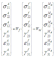
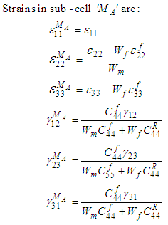
an  represent the axial strain tensor and engineering shear strain components respectively. Note that in all of these symbols the superscript ‘*’ corresponds to one of the following sub cells: fiber f, matrix MA, matrix B or part A and for the occasions in which this superscript is missing, the whole RVC values are being represented. The sub-cells f and MA in part A, are subjected to iso-strain boundary conditions in directions 11, 22, and 12 and iso-stress boundary conditions in directions 23, 33, 31 (as shown in figure 2). Hence the homogenized stresses and strains in part A are represented by the following relations:
 | Figure 2. A schematic illustration of the loading and boundary conditions on Part A |
 | (2a-2f) |
 | (3a-3f) |
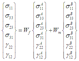
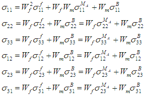
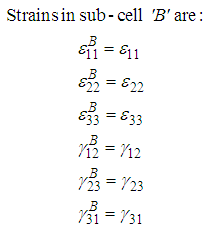
As shown in figure 3, the sub-cell B and part A, are subjected to iso-strain boundary conditions in the 11, 33, 23 and 31 directions and iso-stress boundary conditions in the rest of the directions.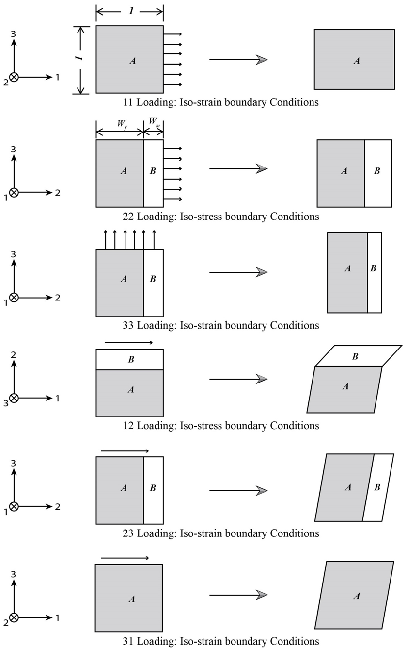 | Figure 3. A schematic illustration of the loading and boundary conditions on the RVC |
The homogenized stresses and strain in the unit cell are hence given by the following equations: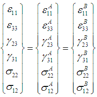 | (4a-4f) |
 | (5a-5f) |
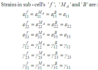
Based on the parallel-series assumptions presented in equations (2) – (5), it is possible to eliminate the intermediate sub-cell A and express the stresses and strains of the RVC in terms of the corresponding constituent sub-cell’s (f, MA and B):For Strains: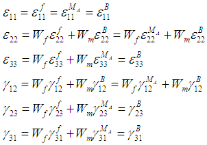 | (6a-6f) |
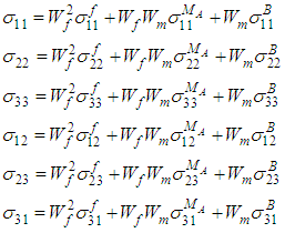
For Stresses: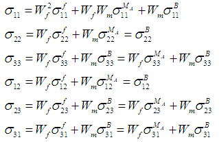 | (7a-7f) |
We have 18 unknowns of strains which correspond to components in each sub-cell (f, MA and B). However, since the average strains in the RVC are known (provided by main FE program), the number of unknowns reduce to 10 with the help of equations provided in (6). Solving for these unknowns becomes necessary in order to calculate the stresses in the RVC. The next section focuses on doing just this.
4. Constitutive Relations of the Micro-mechanical Model
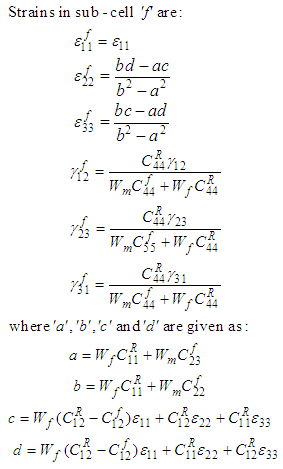
The RVC and the intermediate sub-cell ‘A’ are heterogeneous in nature. However, the base sub-cells (f, MA and B) are considered to be homogenous. The fiber is assumed to be transversely isotropic with the axis of transverse isotropy along the corresponding fiber axis (which is 1-direction for this case). Constitutive relations of the fiber after applying the known values of strain given in equations (6) are:Fiber Sub-Cell (f):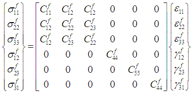 | (8a-8f) |
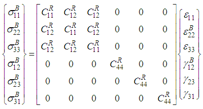
Where,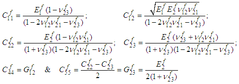
 is the stiffness in the axial directions (i.e., subscript
  ) whereas
  are the poisson’s ratio and the stiffness in the shear directions (i.e., subscript
 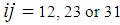 ). The matrix material is assumed to be isotropic and hence the constitutive relations of the sub-cells (MA and B) after applying the known strains from equation (6) are:Matrix Sub-Cell (MA):
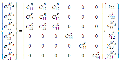 | (9a-9f) |
Matrix Sub-Cell (B):
 (10a-10f)Where,
 The elastic stiffness constants for sub-cells MA and B are the same since they are made out of the same resin material; hence these constants are equivalently represented by the super-script R in the equations (9) and (10). The unknown strains in equation (8), (9) and (10) are denoted by the super-scripts ‘f’ ‘MA’ ‘B’. Hence, in order to calculate the effective RVC stresses it is essential to solve for the following sub-cell strains (10 in total):
 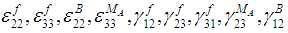 and
and  .From equation (3c), we have the following relation,
 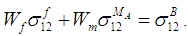 Substituting the relations from (8d) and (9d) into this equation, the shear strain
  can be expressed in terms of
  (as shown in (11a)), which can then be used in equation (6d) to solve for

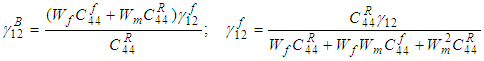
 (11a-11b)Next, using the relations given in (2d), (8d) and (9d), the shear strain
  can be expressed in terms of
  as shown in equation (12a). This can then be used to solve for
  by substituting (12a) in equation (6d).
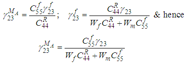
 (12a-12c)Since the boundary conditions between the sub-cells for the components in directions 23 and 31 are the same, the procedure for calculating the unknown strains
  and
and  are similar. Utilizing equations (8f), (9f) in (2f), the shear strain
  can be expressed in terms of
  (as shown in (13a)), which can then be used in equation (6f) to solve for

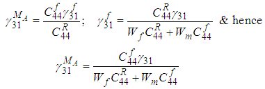
 (13a-13c)Equations (11) - (13) help reduce the number of unknowns to 4, i.e.,
  and
and  . Furthermore,
  can be expressed in-terms of
  and
and  by using (8c) and (9c) in (2e).
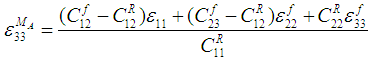 | (14) |
Similarly, using equations (8b), (9b), (10b) and (14) in (7b),  can be expressed in-terms of
  and
and  as shown below:
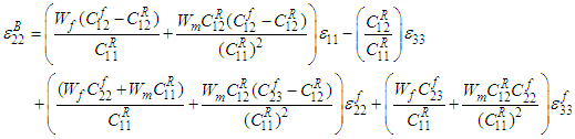 | (15) |
Equation (14) can be further used in (6c) to generate an equation in  and
and  as shown below:
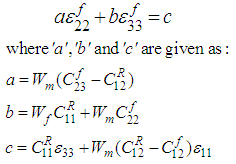 | (16) |
Similarly, using equation 15 in (6b) helps generate the following equation: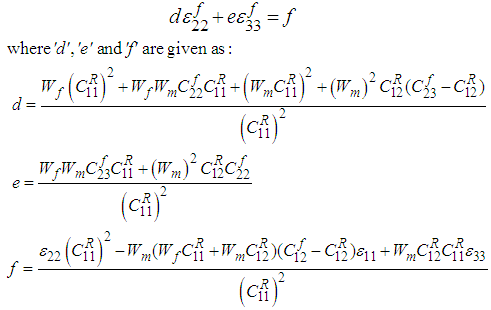 | (17) |
Values  are constants whereas
  can be easily calculated since the average RVC strains are provided by the Finite Element solver at each time step. Lastly, the linear equations (15) and (16) can hence be solved to calculate
  and
and 
 | (18) |
Thus, the strains in all 3 constituent sub-cells are available at this point, which can then be used in equations (8), (9) and (10) and subsequently in equations provided in (7) to calculate the average stresses in the RVC.
5. Results and Discussion
The micro-mechanical equations discussed in the previous section (Current Model), along with the numerical models discussed in the [6] and [4], [5] (Numerical Models 1 and 2 respectively) have been implemented as user material subroutines (UMAT) in LS-DYNA. All three micro-models use the same homogenization scheme; however, employ different sub-cell boundary conditions.Ÿ Current (Curr.) Model: Numerical Model based on physically viable sub-cell boundary conditions (Section 4): ο Sub-cell A: Iso-strain b.c between fiber (‘f’) and Matrix (‘MA’) sub-cells in 11, 22, and 12 directions and Iso-stress b.c in 33, 23 and 31 directions.ο Total RVC: Iso-strain b.c between sub-cell (‘A’) and sub-cell (‘B’) in 11, 33, 23 and 31 directions and Iso-stress b.c in 22, 12 directions.Ÿ Numerical (Num.) Model 1: Numerical Model based on the sub-cell boundary conditions used by Tabiei and Babu [6]:ο Sub-cell A: Iso-strain b.c between fiber (‘f’) and Matrix (‘MA’) sub-cells in all directions.ο Total RVC: Iso-strain b.c between sub-cell (‘A’) and sub-cell (‘B’) in all the directions.Ÿ Numerical (Num.) Model 2: Numerical Model based on the sub-cell boundary conditions used by Tabiei and Chen, Tabiei and Yi [4], [5]:ο Sub-cell A: Iso-strain b.c between fiber (‘f’) and Matrix (‘MA’) sub-cells in 11 and Iso-stress b.c in 22, 33, 12, 23 and 31 directions.ο Total RVC: Iso-strain b.c between sub-cell (‘A’) and sub-cell (‘B’) in all the directions.For the micro-mechanical relations provided in [5] and [6], the in-elastic behavior of the resin has been taken into account. However, since the current work focuses on studying only the elastic constants, it would be apt to derive these equations just for an elastic resin material. Appendix ‘A’ provides the elastic strains of the sub-cells and the constitutive response of the RVC based on the boundary conditions considered in [4] or [5] and [6]. These relations have been derived based on the procedure highlighted in the previous section.
5.1. Analytical Models
In an effort to accurately predict the elastic properties of composite materials based on the constituent properties, a wide range of analytical micro-mechanical models have been discussed in literature over the last century. Younes et al. [7] reviewed some of the most known, readily available analytical models and discussed their performance. The investigated models belonged to the following categories: 1. Phenomenological Models: Rule of Mixture (ROM) / Inverse Rule of Mixture (IROM).2. Semi-empirical Models: Modified Rule of Mixtures (MROM), Halpin-Tsai model and Chamis model [8].3. Elasticity approach Models (EAM): Hashin-Rosen [9] composite cylinder assemblage model (CCA) coupled with Christensen model [10].4. Homogenization Models: Mori-Tanaka Model, Self-Consistent model (S-C) and Bridging model [11], [12]. The Chamis model has been observed to yield good results for all the cases studied. Whereas, the rest of the models have been observed to predict elastic properties well for only certain cases. In this study, the best working model in each of these categories (ROM / IROM, Chamis, EAM and Bridging) has been compared against the numerical models. The motive for using some of the widely popular analytical methods is that in the absence of experimental data, they help decide how good the numerical prediction really is. In addition, since the constituent properties and some of the available experimental data have been collected from various sources, there is a good chance that that the results might not completely match. Therefore, the analytical results help generate confidence in the data generated by the numerical models as there may be abnormal data points in the experimental values.
5.2. Numerical FE Model
Numerical FE models have been widely used in predicting the mechanical properties of composites. For the current case, a single element model (Figure 4) has been subjected to a displacement constant ‘c’ on various faces, with different boundary conditions (as shown in Table 1).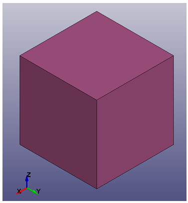 | Figure 4. An un-deformed single solid element FE model |
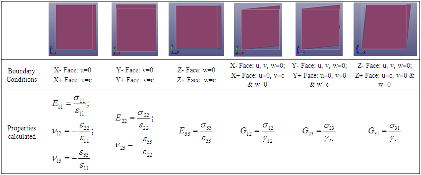 | Table 1. Deformed state’s, Boundary Conditions on the X, Y and Z faces of the Solid Element |
A total of six simulations have been conducted for each lamina considered with the value of the displacements (u, v and w) varying depending on the property that is being calculated. The stresses and strains used in these property calculations are obtained from the integration point at the center of the element.
5.3. Comparative Study, Analysis and Discussion
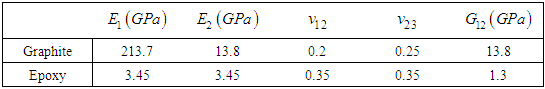
In this section a comparison of the analytical models and numerical results with available experimental data is presented. A total of 6 composite laminas have been studied and the constituent properties of these laminas have been provided in Table’s (2) – (7):Table 2. Properties of Graphite/Epoxy (AS/3501) [4]
 |
| |
|
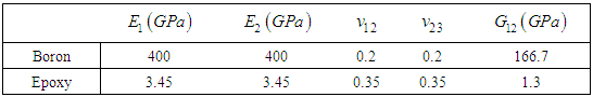
Table 3. Properties of Boron/Epoxy (B4/5505) [4]
 |
| |
|
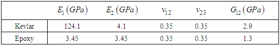
Table 4. Properties of Kevlar/Epoxy [4]
 |
| |
|
Table 5. Properties of Glass/Epoxy [13]
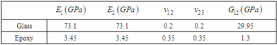 |
| |
|
Table 6. Properties of Carbon/Epoxy [12]
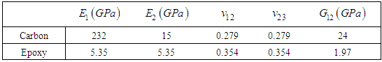 |
| |
|
Table 7. Properties of Polyethylene/Epoxy [14]
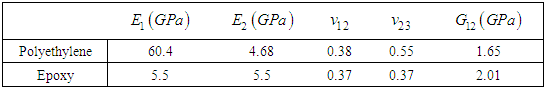 |
| |
|
The glass and boron fibers mentioned above are considered to be isotropic whereas the rest of the fibers are transversely isotropic in nature. In addition, the epoxy resin in all the cases is assumed to be isotropic as well. The accurate prediction of the transversal and shear modulus has presented a major challenge for researchers over the years. In fact, many analytical models belonging to different micromechanics approaches have solely been proposed to address these shortcomings. In the following sections, emphasis has been placed on studying the effect of numerical methods in predicting the transversal (22 direction) and shear moduli (in-plane: 23 direction and out-of-plane: 12 direction). Each numerical method has been analyzed over 4 volume fractions for each composite lamina. Hence, a total of: 3 numerical methods * 6 composites * 4 volume fractions * 6 single element cases (Table 1) = 432 runs, have been carried out and examined in this study. Since it wouldn’t be viable to present and discuss all the 9 elastic constants for the 6 composites that have been investigated (which would result in 9*6=54 figures), a table comprising of all 9 elastic constant predictions has been presented for each lamina for the most commonly used volume fraction. Correspondingly, the transverse and shear moduli have been presented and compared as plots for all 4 volume fractions considered.
5.3.1. Graphite/Epoxy (AS/3501)
Table 8 comprises of all 9 elastic constants that have been predicted using the fore-mentioned numerical models and the typical experimental predictions for a volume fraction of 0.66.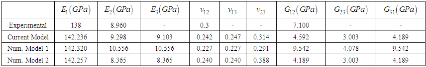 | Table 8. Elastic properties predicted for Graphite/Epoxy-AS/3501 lamina, Volume Fraction = 0.66 |
Owing to the relative simplicity of coding the analytical methods in comparison to the numerical methods, the elastic constants have been predicted at various volume fractions ranging from 0 to 1 for the 4 analytical methods considered. It can be observed from Figure 5, that all the numerical methods predict the stiffness in the fiber direction quite accurately. In fact, this has been observed to be a common trend in all the discussed composites. It can also be said that the current micro-mechanical model does quite well in predicting the transverse modulus (Figure 6) when compared to other numerical methods. The shear modulus (Figure 7) is slightly under-predicted by the current numerical model and numerical model 2, however since they agree quite well with the analytical methods for all the volume fractions it could suggest an anomaly in the experimental data.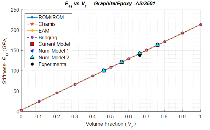 | Figure 5. Analytical, numerical and experimental results for Graphite/Epoxy ( in terms of in terms of  ) ) |
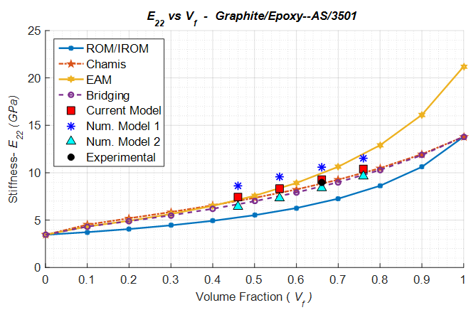 | Figure 6. Analytical, numerical and experimental results for Graphite/Epoxy ( in terms of in terms of  ) ) |
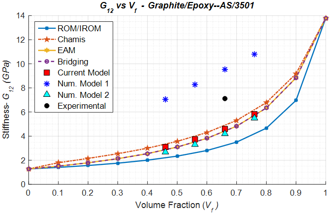 | Figure 7. Analytical, numerical and experimental results for Graphite/Epoxy ( in terms of in terms of  ) ) |
5.3.2. Boron/Epoxy (B4/5505):
Based on the results shown in Table 9, it can be said that the current numerical model and numerical model 2 have been able to predict the transverse and shear moduli acceptably in comparison to the experimental results.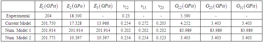 | Table 9. Elastic properties prediction for Boron/Epoxy (B4/5505) lamina, Volume Fraction = 0.5 |
Numerical Model 1 however has been observed to significantly overestimate both the transverse and shear moduli. This can be accredited to a deadly mixture of high transverse/shear modulus of the boron fibers and the use of iso-strain boundary conditions throughout. The current model accurately predicts the transverse modulus emphasizing the importance of correct sub-cell boundary conditions.From figures 8 and 9, for the volume fraction cases in which the experimental data wasn’t available, it is evident that the current numerical model and the numerical model 2 calculate moduli values closer to the analytical models.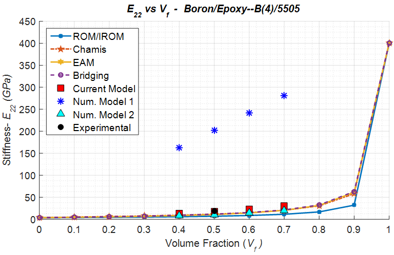 | Figure 8. Analytical, numerical and experimental results for Boron/Epoxy ( in terms of in terms of  ) ) |
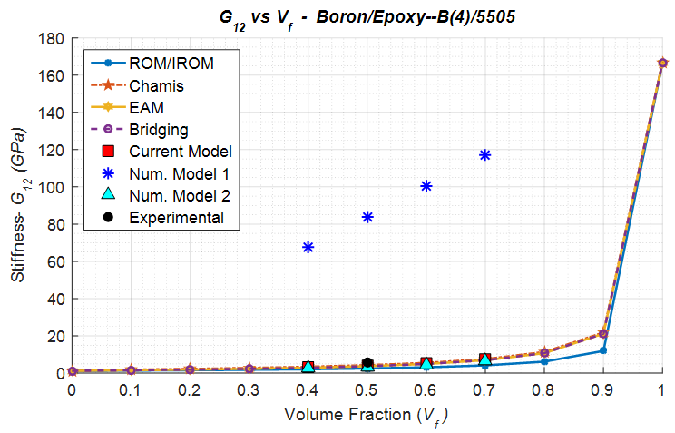 | Figure 9. Analytical, numerical and experimental results for Boron/Epoxy ( in terms of in terms of  ) ) |
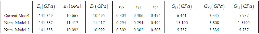
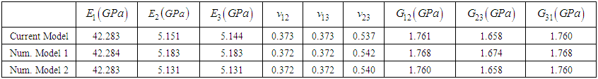
5.3.3. Kevlar/Epoxy
Based on the elastic constants shown in Table 10, it can be said that all numerical models perform in a similar manner and predict good results in comparison to the experimental data.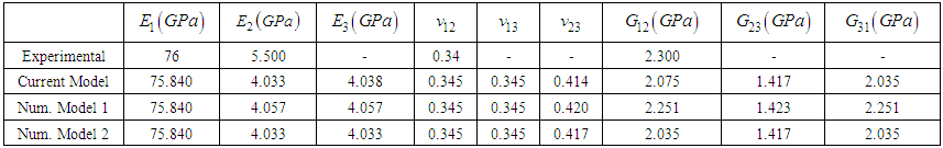 | Table 10. Elastic properties prediction for Kevlar/Epoxy lamina, Volume Fraction = 0.6 |
 | Table 11. Elastic properties prediction for Glass/Epoxy lamina, Volume Fraction = 0.43 |
 | Table 12. Elastic properties prediction for Carbon/Epoxy lamina, Volume Fraction = 0.6 |
 | Table 13. Elastic properties prediction for Polyethylene/Epoxy lamina, Volume Fraction = 0.67 |
In contrast to the axial and shear moduli, the transverse shear modulus is slightly under predicted for all 3 numerical cases. The numerical results agree quite well with the Bridging analytical model in the transverse direction (Figure 10) and the Chamis analytical model in the shear direction (Figure 11).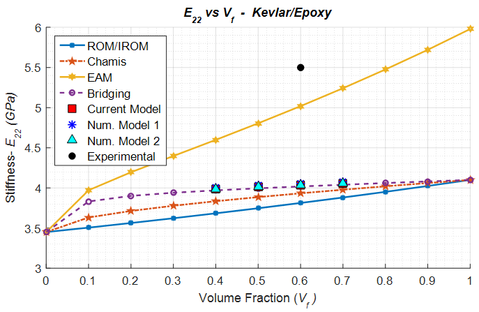 | Figure 10. Analytical, numerical and experimental results for Kevlar/Epoxy ( in terms of in terms of  ) ) |
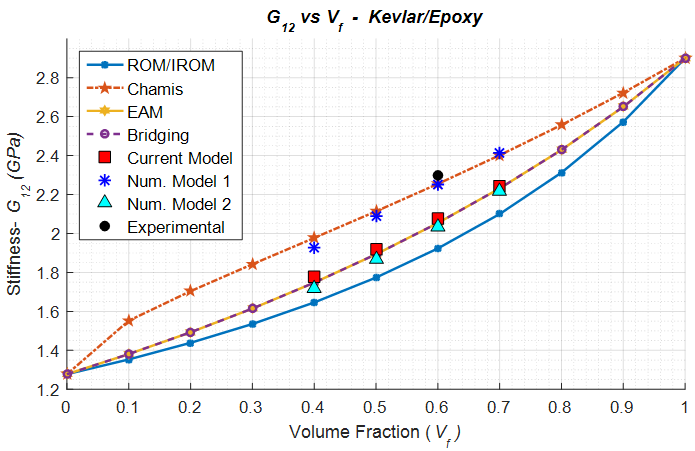 | Figure 11. Analytical, numerical and experimental results for Kevlar/Epoxy ( in terms of in terms of  ) ) |
5.3.4. Glass/Epoxy
The transverse modulus (Figure 12) calculated by the current numerical model and numerical model 2 have been observed to be closer to the experiments whereas numerical model 1 significantly over predicts. The trends observed for this particular case are very similar to what has been seen for the boron/epoxy case and is attributed to the presence of isotropic fibers.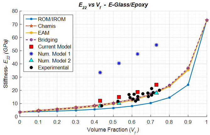 | Figure 12. Analytical, numerical and experimental results for Glass/Epoxy ( in terms of in terms of  ) ) |
5.3.5. Carbon/Epoxy
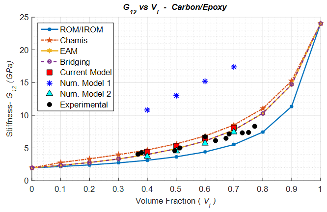
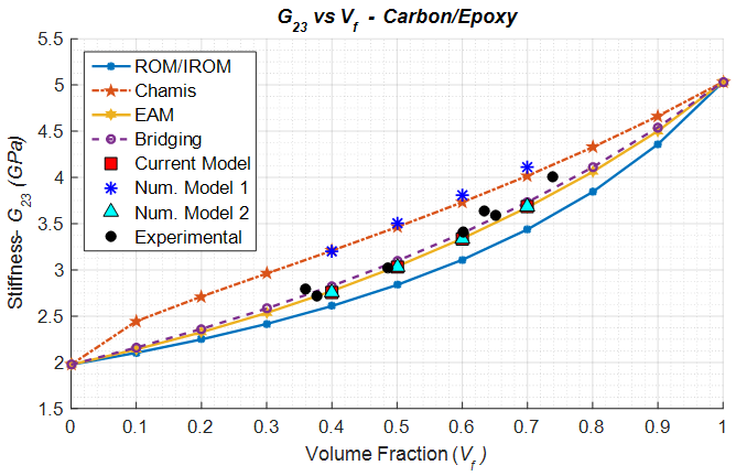
Transverse modulus (Figure 13) predictions have been observed to be fairly accurately for all 3 numerical models. The numerical model 1 consistently over predicts the shear moduli (Figure 14) in both the shear directions; whereas the current numerical model and numerical model 2 have been observed to do well once again.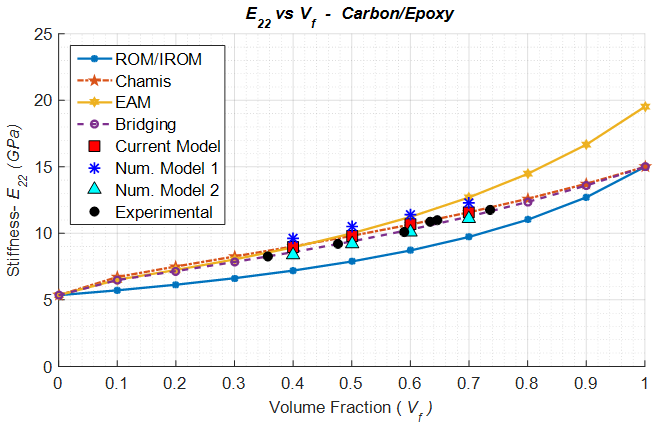 | Figure 13. Analytical, numerical and experimental results for Carbon/Epoxy ( in terms of in terms of  ) ) |
 | Figure 14. Analytical, numerical and experimental results for Carbon/Epoxy ( in terms of in terms of  ) ) |
 | Figure 15. Analytical, numerical and experimental results for Carbon/Epoxy ( in terms of in terms of  ) ) |
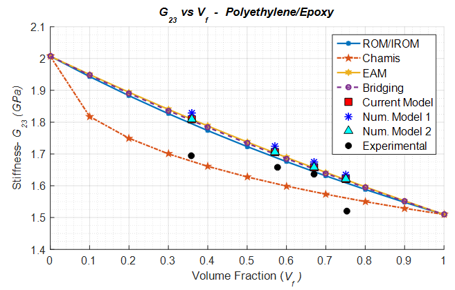
5.3.6. Polyethylene/Epoxy
Polyethylene/Epoxy composite lamina is considered a special case as the young’s modulus of the epoxy is higher than that of the transversal modulus of the fibers. Due to this distinctive behavior, the ROM / IROM analytical model which has served as a lower bound to the transverse and shear moduli predictions so far has been replaced by the Chamis model. In comparison to the experimental results, the Chamis model has been observed to do well for high fiber volume fraction cases. However, nearly all other analytical models struggle to predict the transverse and shear modulus accurately. All 3 numerical models accurately predict the in-plane shear modulus (Figure 17); however slightly over-predict the transverse (Figure 16) and the out-of-plane shear moduli (Figure 18).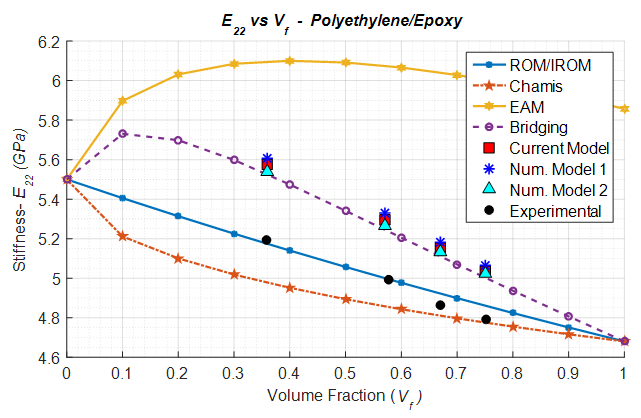 | Figure 16. Analytical, numerical and experimental results for Polyethylene/Epoxy ( in terms of in terms of  ) ) |
 | Figure 17. Analytical, numerical and experimental results for Polyethylene/Epoxy ( in terms of in terms of  ) ) |
 | Figure 18. Analytical, numerical and experimental results for Polyethylene/Epoxy ( in terms of in terms of  ) ) |
6. Conclusions
In this study, a micro-mechanical material model based on physically viable boundary conditions has been derived. This model along with similar models (different boundary conditions) from the literature has been evaluated for the elastic properties. The results have been compared against popularly known analytical micromechanical models, as well as available experimental data for six different UD composites: Graphite/Epoxy (AS/3501), Boron/Epoxy (B4/5505), Kevlar/Epoxy, Glass/Epoxy, Carbon/Epoxy and Polyethylene/Epoxy. It has to be noted that the studied cases cover isotropic fibers (glass, boron) as well as transversely isotropic fibers (graphite, kevlar, carbon and polyethylene). The analyses of the compared results show clearly that all numerical models show a very good agreement for the longitudinal Young’s modulus  and major Poisson’s ratio
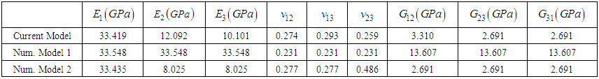
  Numerical Model 1 on the other hand, has been consistently observed to over-predict the transverse and shear modulus. Even though there have been cases where this model does equivalently well in comparison to the other numerical models, it would be fair to say that this model cannot be used to study composites with isotropic fibers. The current numerical model and numerical model 2 have been fairly accurate in predicting the transverse and shear moduli (out-of-plane) for most cases. For the cases in which these models failed to match the experimental values, they have been close to the predictions of a majority of analytical models which inspires confidence in the validity of the boundary conditions used. When comparing the current numerical model against numerical model 2, it can also be said that the shear moduli (out-of-plane) estimated by the current numerical model is much closer to the experimental value. It is worth mentioning that, both models work equally well for composites with isotropic fibers as well as transversely isotropic fibers. The transverse moduli (directions 22 and 33) of the composite, predicted by the current Model are no longer the same as a consequence of using different boundary conditions in each of these directions during model development. This is unlike what has been observed in numerical models 1 and 2. For the cases where experimental data was available it has been observed that the current numerical model and numerical model 2 accurately predict the in-plane shear
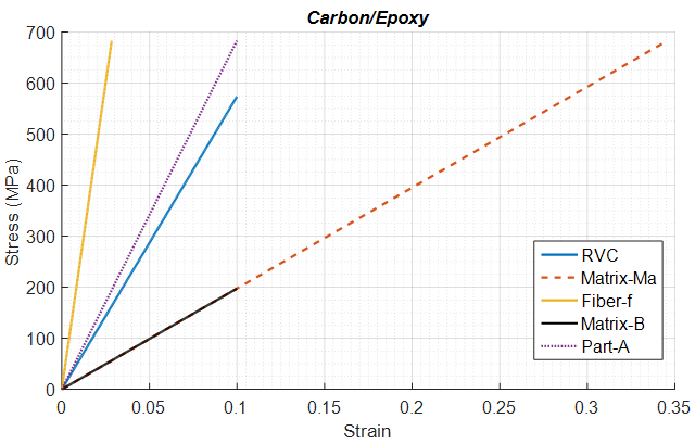
  modulus.It is important to understand that despite closer RVC moduli predictions made by the current numerical model and numerical model 2 for most cases, using correct boundary conditions is still key for future studies since each constituent sub-cell experiences a different amount of stress or strain and this plays a crucial role once in-elastic behavior or failure criteria are introduced. As an example, a single element RVC model (with Carbon/Epoxy material properties) subjected to a fixed amount of shear strain is studied for both these models (Figures 19 and 20).
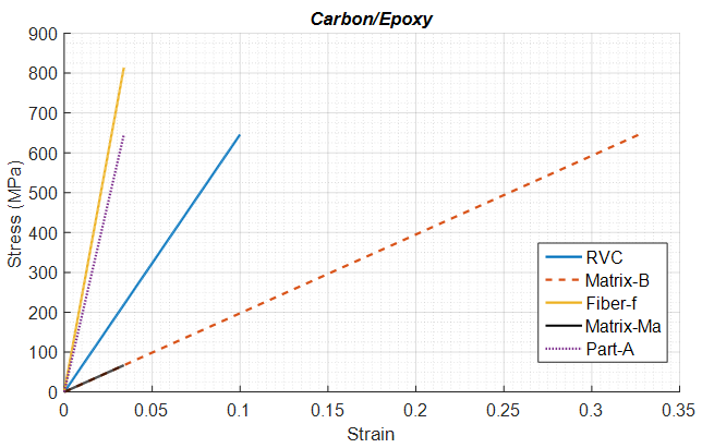 | Figure 19. Shear stress vs Shear strain predicted by Current Model; Volume Fraction=0.6 |
 | Figure 20. Shear stress vs Shear strain predicted by the Numerical Model 2; Volume Fraction=0.6 |
A key advantage of micro-mechanical models is that, depending on the failure mode, the stresses/strains calculated in each constituent (fiber and matrix) can be related to a simple failure model and depending on this failure criterion proper degradation of strength is achieved. In the current example, it is quite evident that a selected sub-cell experiences significantly different stress/strain behavior for the current numerical model and numerical model 2. Thus, when coupled with a simple failure model it would fail differently as well. This emphasizes the need for use of physically correct boundary conditions in the micro-model.Lastly, as a conclusion from this study, it can be said that the proposed micro-mechanical material model performs very well in correctly predicting the elastic constants of a wide range of composite laminas.
Appendix A
Boundary conditions discussed in Tabiei et al. [4] considers the sub-cells f and MA in part A, to be in parallel (iso-strain) in direction: 11 and in series (iso-stress) in directions: 22, 33, 12, 23 and 31. All the components of sub-cell B and part A, are then considered to be acting in parallel (iso-strain). This results in the following equations:For Strains:
 (A.1.a-f)For Stresses:
 (A.2.a-f)It can be easily observed that there are 5 unknowns to be solved for:
  and
and  . Using the constitutive relations of the constituents, each of these unknowns can be solved for using the procedure discussed in Section 4. The elastic strains in each sub-cell in-terms of the known values can hence be given by the following relations:
 (A.3.a –f)
 (A.4.a –f)
 (A.5.a –f)Thus, the strains in all 3 constituent sub-cells, can then be used with the sub-cell stiffness components (shown in equations (8), (9) and (10)) to calculate the corresponding stresses. These constituent stresses are then used in equations (A.2) to calculate the average stresses in the RVC.Boundary conditions discussed in Tabiei et al. [6] result in even more straight-forward equations for the sub-cell strains as they are assumed to be in parallel (iso-strain) in all directions. Hence the elastic strains for each sub-cell are given by the following relations:
 (A.6.a –f)Subsequently, the average stresses in the RVC are:
 (A.7.a –f)
Appendix B
Nomenclature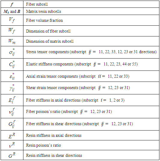 Superscript:
References
| [1] | LS-DYNA Keyword User’s Manual, Volume I & II, LS-DYNA R8.0, Lawrence Livermore Software Technology Corportation(LSTC), 2015. |
| [2] | Adams, Donald F., and David A. Crane. "Finite element micromechanical analysis of a unidirectional composite including longitudinal shear loading."Computers & structures 18.6 (1984): 1153-1165. |
| [3] | Pecknold, D. A., and S. Rahman. "Micromechanics-based structural analysis of thick laminated composites." Computers & structures 51.2 (1994): 163-179. |
| [4] | Tabiei, Ala, and Quing Chen. "Micromechanics based composite material model for crashworthiness explicit finite element simulation." Journal of Thermoplastic Composite Materials 14.4 (2001): 264-289. |
| [5] | Tabiei, Ala, Weitao Yi, and Robert Goldberg. "Non-linear strain rate dependent micro-mechanical composite material model for finite element impact and crashworthiness simulation." International Journal of Non-Linear Mechanics 40.7 (2005): 957-970. |
| [6] | Tabiei, Ala, and S. Babu Aminjikarai. "A strain-rate dependent micro-mechanical model with progressive post-failure behavior for predicting impact response of unidirectional composite laminates." Composite Structures 88.1 (2009): 65-82. |
| [7] | Younes, Rafic, et al. Comparative review study on elastic properties modeling for unidirectional composite materials. INTECH Open Access Publisher, 2012. |
| [8] | Chamis, Christos C. "Mechanics of composite materials: past, present, and future." Journal of Composites, Technology and Research 11.1 (1989): 3-14. |
| [9] | Hashin, Zvi, and B. Walter Rosen. "The elastic moduli of fiber-reinforced materials." Journal of applied mechanics 31.2 (1964): 223-232. |
| [10] | Christensen, R. "A critical evaluation for a class of micromechanics models Journal of the Mechanics and Physics of Solids. 38." (1990): 379-404. |
| [11] | Huang, Zheng-Ming. "Simulation of the mechanical properties of fibrous composites by the bridging micromechanics model." Composites Part A: applied science and manufacturing 32.2 (2001): 143-172. |
| [12] | Huang, Zheng-ming. "Micromechanical prediction of ultimate strength of transversely isotropic fibrous composites." International journal of solids and structures 38.22 (2001): 4147-4172. |
| [13] | Shan, Hui-Zu, and Tsu-Wei Chou. "Transverse elastic moduli of unidirectional fiber composites with fiber/matrix interfacial debonding." Composites Science and Technology 53.4 (1995): 383-391. |
| [14] | Wilczyński, A. P., and J. Lewiński. "Predicting the properties of unidirectional fibrous composites with monotropic reinforcement."Composites science and technology 55.2 (1995): 139-143. |
| [15] | Aboudi, Jacob. "Micromechanical analysis of the strength of unidirectional fiber composites." Composites science and technology 33.2 (1988): 79-96. |

 Abstract
 Reference
 Full-Text PDF
 Full-text HTML