Benjamin Fischer1, Bernhard Horn2, Christian Bartelt1, Yannick Blößl2
1Institute for Computer Science, Clausthal University of Technology, Clausthal, Germany
2Institute for Carbon Composites, Technische Universität München, Munich, Germany
Correspondence to: Benjamin Fischer, Institute for Computer Science, Clausthal University of Technology, Clausthal, Germany.
| Email: |  |
Copyright © 2015 Scientific & Academic Publishing. All Rights Reserved.
Abstract
The manufacturing of composite structures is expensive due to high material cost and the amount of manual labor needed. Current manufacturing technologies, e.g. filament winding, braiding or fiber placement technologies are offering a possibility of automated manufacturing to lower these costs. Nevertheless, these technologies are limited when it comes to structures with complex fiber architecture and small geometries. A new approach to overcome these limitations is the fiber patch placement technology. The preform of a composite structure is built up with small and dry fiber patches in a sequential order. Fiber discontinuities are necessarily occurring between two patches and are influencing the mechanical properties. To optimize strength of the composite those discontinuities have to be distributed within the preform. With increased number of patches, the number of combinations of patch positions is increasing significantly. This paper presents a method based on an ant colony algorithm for an efficient calculation of an optimized distribution, which enables to use the potential of patched laminates.
Keywords:
Ant Colony Algorithm, Fiber Patch Placement, Automated Optimization, Composite Manufacturing
Cite this paper: Benjamin Fischer, Bernhard Horn, Christian Bartelt, Yannick Blößl, Method for an Automated Optimization of Fiber Patch Placement Layup Designs, International Journal of Composite Materials, Vol. 5 No. 2, 2015, pp. 37-46. doi: 10.5923/j.cmaterials.20150502.03.
1. Introduction
The main cost drivers in current manufacturing of composite materials are material cost and the amount of work due to a high amount of manual labor. Significant reduction in manufacturing cost of fiber material or impregnation resin are limited whether the manufacturing process still offer a high potential for cost reduction especially with lowering of fiber consumption or fiber waste [1]. One possibility to reach this goal is a load path optimized design of composite parts, for example with “variable stiffness” approach [2-4]. A decrease in the amount of work can be achieved by increasing the amount of automation. This requires automatized and material saving manufacturing processes.Filament winding, braiding or fiber placement technologies are already state of the art in industrial serial production due to their high grade of automation. The drawbacks of these technologies are limitations when it comes to small and complex geometries. For hollow structures, braiding and filament winding are often the most suitable technologies, as long as the geometry has a convex shape. Strong concave surfaces cannot be covered [5]. The fiber tension leads to a bridging effect, which causes the roving to overstretch the surface instead of following the geometry. This restricts the variety of producible composite parts to convex geometries or requires further forming steps. If convex and concave areas are alternating, the fiber placement processes are beneficial. The processes are classified regarding their raw material used (fiber tape, fiber roving, fiber patch). For geometries with lower complexity e.g. an airplane body shell or wing section, the automated fiber placement process (AFP) is often used [6]. For this technology limitations are reached when it comes to a small radius of curvature [7]. The in-plane bending of tapes leads to fiber undulation on the inner side of the tape. This steering limits are strong dependent on tape width, track length and tack of the tape [9]. Blom gives values for the minimum curvature from 635 mm (tape width: 1/8 in) to 8890 mm (tape width: 1/2 in) [8]. This shows that with increasing tape width the minimum curvature increases strongly and therefore only parts with less complex fiber architecture are becoming possible. The tailored fiber placement process (TFP) uses fiber rovings, which are fixed onto a surface by sewing. Small radii of curvature are often leading to uneven fiber distribution over the roving cross section and to imprecise fiber placement [9]. This process additionally requires a downstream forming step to create three-dimensional structures, which increases production time and cost. The limitations of the presented processes lower the lightweight potentiality of carbon fiber materials due to the fact that load path optimization cannot be fully exploited for small and complex (small radii of curvature and complex fiber architecture) parts. The advantage of using fiber patches to increase mechanical properties was shown by Götz [10]. Unidirectional glass fiber tapes were used to improve notch behavior and a multi linearization method was developed to increase maximum strength of a composite. Another new process in this field is called Tailored Patch Placement. Thermoplastic fiber patches are placed on existing structures as a local reinforcement in a load path optimized way [11]. For the production of parts with high complexity and small size, the fiber patch placement process has been developed. Moreover, it was been developed to apply local reinforcements. It combines the common preform steps, material supply, cutting and draping extended by a quality inspection system. A fast moving pick and place robot places unidirectional long fiber patches on a tool with a high degree of freedom in terms of position and orientation. The patches are cut out of spread fiber tape without cutting waste to decrease the amount of fiber consumption. In contrast to the processes, which were introduced at the beginning of this paper, no limitation in radii of curvature exists because a radius is covered by line of patches instead of a continuous fiber. This is leading to very high design flexibility. A comparison between continuous fiber tapes and long fiber patches (rectangular patch geometry) is shown on Figure 1. When using rectangular patches gaps and overlapping areas are resulting which affects the final composite properties. Those can be eliminated by varying the cutting geometry, e.g. round shaped edges. For the following study, those characteristics are not relevant and are therefore not further discussed.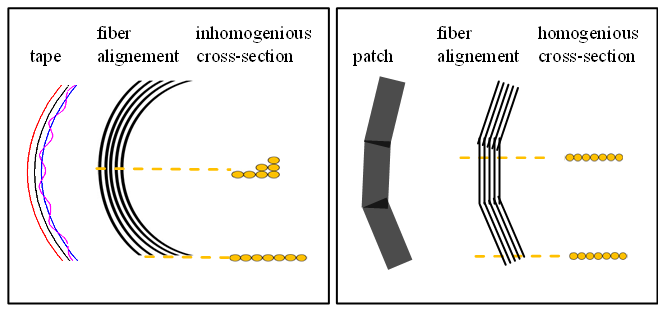 | Figure 1. Difference between fiber tape and fiber patch |
This high placement flexibility is leading to higher design effort needed because the distribution and form of the discontinuity has the highest impact on the mechanical parameters achievable, e.g. maximum strength. The layup of a typical FPP-laminate is shown in Figure 2. Each layer consists of a patch pattern depended amount of sub layers. Those sub layers themselves are consisting of lines of patches. This quasi-continuous line is called a patch line. Between two patches therefore a discontinuity occurs. Through shifting of sub layers relative to each other the position of the discontinuity in the laminate and thereby the mechanical properties can be tailored. 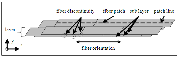 | Figure 2. Schematic build-up of a patched laminate |
Due to the newness of the technology, those effects are not fully understood or investigated. The influence of a discontinuity on the maximum strength and its dependence on the thickness of each sub layer was further investigated by Wisnom [12]. With decreasing thickness of a sub layer, an increased maximum strength was identified. An approach of the influence of the patch pattern on the expected strength of the composite was presented by Mayer [13]. He postulated that the discontinuities have to be distributed with maximum distance to each other. This relation is illustrated on Figure 3. For layup design no. 1, the discontinuities are positioned on top of each other, forming a straight line. The maximum strength is thereby defined by the mechanical properties of the resin system. Compared to this, in design no.4 the discontinuities are shifted relative to each other to minimize the difference in strength between layup of continuous fibers and fiber patches (cf. [13]). 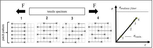 | Figure 3. Influence of patch pattern on the estimated composite strength cf. [12] |
The design of the patch plan, which defines the position of each patch, has to be distinguished from a topological optimization. The challenge of layup design is to distribute the fiber discontinuity where a topological optimization for example focuses on a more efficient material use due to optimized fiber positioning. While the layup design is dependent on a lot of boundary conditions, e.g. amount of patches or patch position, this paper presents a new approach to calculate the best design automatically. Therefore, a formula to predict the strength of a patched composite has been developed which bases on scientific findings on the behavior and the failure mechanism of patched laminates. The solution space for this kind of problem (independent shifting of the patches on each patch line) is very large. Typically those problems are mathematically solved with heuristic algorithms [14]. Due to their structure, two heuristic algorithms (the generic algorithm and the ant algorithm) were closer investigated. The first one finds a better solution by combination of previous solutions where the second one finds a better solution by regarding previous results [15]. Those initial solutions are not available at the beginning of the calculation and would have to be determined in a time-consuming preliminary stage. The ant algorithm therefore can produce meaningful results without this step and was therefore chosen in this investigation to keep the amount of calculation effort as low as possible.
2. Fitness Function
Due to the sequential buildup of a preform with fiber patches, the presented problem concerning the distribution of fiber discontinuities in the laminate occurs. This discontinuity in fiber path is affecting the mechanical properties of the compound and has to be considered while designing the patch layup. The optimization itself requires relations to describe the influence of the patch pattern on the mechanical properties. Like already described in the introduction, different patch patterns are leading to different failure mechanisms and strength if a tensile force applies. If a patch line is under tension force, load has to be redirected from one layer to the bordering layer by shear stresses. The resin rich discontinuity cannot transfer the load sufficiently. The overlapping of the layers defines the area, which is available to redirect the load. Depending on the arrangement of the patches, different configurations show a better or worse behavior. For FPP-laminates with a unidirectional fiber orientation under uniaxial load in fiber direction, the resulting strength can be traced back to the geometrical properties of the patch overlap.As an example, Figure 4 shows an exemplary patch layup with two sub layers. The sub layers are shifted to each other, which is leading to a distribution of the fiber discontinuity in the laminate. Within a sub layer, the patches have no gaps or overlaps. The illustrated geometrical parameters are defining the patch coverage in the upper layer with patches in the lower layer (dotted red frame). In this case, four patches of the upper layer cover the patch in the lower layer. The overlapping lengths are labeled with lA and lB. In addition, with the width parameters A and B they are forming the corresponding overlapping area. This is all under the assumption that areas with smaller overlapping length are tend to fail earlier than areas with larger areas if tension force applies. With those geometrical parameters for every patch combination a validation of the laminate quality and therefore a validation optimization of the patch positioning becomes possible. 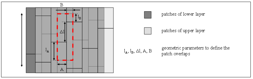 | Figure 4. FPP-Laminate with two sub layer |
Figure 5 sketches the geometrical input data for the qualification function QP of the patch positioning.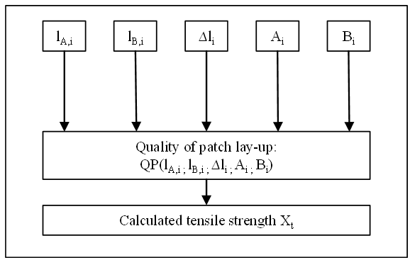 | Figure 5. Input parameter to determine the quality of the patch lay-up |
The relation between the input parameters and the laminate quality is chosen in a way that the resulting QP-value of different patch pattern is correlating with the expected tensile strength in fiber direction Xt. The validation of this relation was proven by comparing results with experimental data of tensile tests with different patch pattern.The manipulation of the patch position in the laminate is leading to new geometrical overlapping parameters and thereby to change in quality parameter QP. The results of this validation are used in the optimization process to find patch positions that are leading to the highest mechanical performance of the composite.
3. Optimization of a Fiber Patch Placement
Based on the described fitness function an algorithm to calculate a good allocation in a reasonable time has been developed.
3.1. Analyze of the Laminate Structure
The preform is divided into layers, which are optimized independently. Every layer consists of sub layers itself, which are containing a specific set of patch lines. Analyzing the structure of the laminate shows, that every patch line can be moved independently to all other patch lines (c.f. Figure 4). Therefore a laminate containing n patch lines, calculated in Equation 1 with l sub layers and pi for the set of patch lines in sub layer i, and a movement in 10 steps for every patch line has 10n possible allocations (see Equation 1). In this set of possible allocations a solution, which satisfy all requirements, has to be found. Because of the size of the set, such a problem cannot be solved by analytic algorithm in an acceptable time, because that kind of problem is NP-hard. It can be compared to the Traveling Salesman Problem, a well-known NP-hard problem [16] with similar constraints.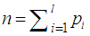 | (1) |
To solve such type of problems, often heuristic algorithms are used, c.f. [17], [18] and [19]. By using a fitness function to get the quality for every allocation, all allocations can be sorted based on their quality. With that sorted list, those algorithms can be used to find those solutions. One kind of these algorithms is called ant colony algorithm and was used in this case.
3.2. Ant Colony Optimization Algorithm
This Chapter describes the class for ant colony algorithms and their application regarding the introduced problem domain.
3.2.1. Ants in Nature
Scientists did research on this algorithm strategy by watching ant colonies. In order to find the shortest way to their food every ant places pheromone while randomly choosing a way to search for food. Following ants can choose a way depending on the intensity of the current pheromone on the ground, or a new way if the intensity is too low. Pheromones lose their intensity over time, therefore if a way is not used for a specific time, all the pheromones are volatilized. Because all ants have nearly the same speed, ants can use a short way to a food source more often than ants, which use a long way in the same period of time. Because of that, the intensity of pheromone is higher on shorter ways than on longer ways. This is why future ants choose the shorter ways more often than the longer ones and that increases the intensity of pheromone on this way even more. As a result, after some time all ants choose the shortest way to the food source and optimize their work by this behavior (c.f. Figure 7). Here the ants are represented as three connected dots. The thickness of the line between food and home represents the pheromone intensity. At the beginning (left path), two ants are on each path because all paths have the same pheromone intensity. AT the end (right path), nearly all ants are on the shortest path (thickest line).
3.2.2. Transformation to an Algorithm
Considering the phenomenon in nature an algorithm can be derived. The problem can be visually illustrated as a graph with edges and vertices containing many paths from start to end (c.f. Figure 6). Each edge has a cost value for using this edge. The goal is to find the shortest way, with the lowest sum of cost of all used edges from start to end.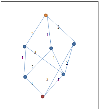 | Figure 6. Example of a graph for searching a path from start to end |
Because of similarities, most information can be transformed directly to the algorithm, e.g. the path with its sections, the length and the ants. The only item, which has to be calculated, is the number of pheromones. Table 1 gives the needed elements for the algorithm and their corresponding equivalent in nature and for this optimization problem. Table 1. Transformation of Terms from Nature to our Algorithm
 |
| |
|
Similar to nature the algorithmic optimization uses a set of fictive ants, which randomly search a path from start to end. After all ants have reached the end vertex, they add a pheromone value to their used edges. The value is the sum of the inverted cost of all used edges, c.f. Equation 2 where ci is the cost of part i of the chosen path.  | (2) |
The shortest way has the highest value. Before adding these values to the pheromones of the edges, the pheromones of all edges have to be volatilized by using a user defined factor. On every vertex, an ant looks at the pheromone of the edges it can choose next. A high pheromone value on an edge lets an ant choose this edge with a high probability.After a short time, nearly all ants use the shortest found path, which is the result of the algorithm and equal to the phenomena in nature.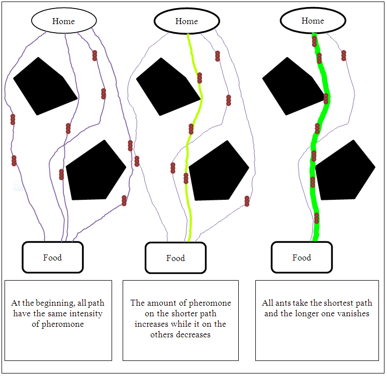 | Figure 7. Path finding of ants in nature over time |
3.2.3. Adaption of the Algorithm to our Problem
A short way of the ant colony is assigned to a good patch allocation of a preform (c.f. Table 1). Because shifting patches on patch lines generates a specific allocation, the decision, which shift should be chosen, can be assigned on which way an ant choose at a crossroad. The algorithm needs a limited number of decisions for every patch line. Therefor a limited number of shifts for every patch line is needed, which means discrete shifts, so called steps. The number of steps can be set for every single optimization of a patch layup plan. The other part of the adaption is writing a specific pheromone function for our problem.
3.3. Pheromone Function
The validation of the optimization algorithm with different examples shows a problem for very small (0<x<1) or very high (e.g. x>1000) values of the fitness function. For very small values the result of the algorithm was very similar to the process of searching an allocation by random and generates similar allocations, because the costs of the chosen parts change only a little. On the other end of the line, one generated allocation can have a much higher value than all other found allocations. From that step, this allocation will be most probably found. Using scale factors for every component to adapt the value from the fitness function is one possible solution to solve that problem. This factor has to be determined empirically. Therefore, the following pheromone function has been generated to adapt the value from the fitness function before using it in the algorithm. Every value from the fitness function from past loops of the algorithm will be kept in a sorted list, c.f. Figure 8. The best 20 percent of the list define a space between 1 and 100 for new pheromone values. The best value gets the value 100 and the worst value of the 20 percent gets the value 1.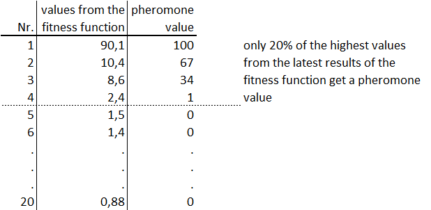 | Figure 8. Example of a pheromone calculation table |
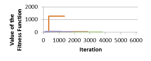
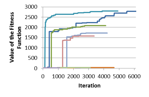
In every loop, the values from the fitness function are compared to the values in the list. According to its position in the list the resulting pheromone value is calculated. The pheromone value will be a value between 1 and 100 if its position is in the best 20 percent of the list. If the value is smaller than the worst value of the best 20 percent of the list, the pheromone value will be zero. This value is used for adapting the pheromone values of the patch lines described above. Then the origin value from the fitness function is inserted in the sorted list and the pheromone values of the list are recalculated. That means that every used value lies between 1 and 100 or has the value 0.Figure 9 and Figure 10 are showing two diagrams with 10 optimizations of the same component in each diagram. The diagram in Figure 9 shows 10 optimizations, where the value of the fitness function is directly been used for adapting the pheromones and the diagram in Figure 10 shows 10 optimization experiments using the pheromone function. The horizontal axis shows the amount of loops and the vertical axis the currently best found quality parameter QP (c.f. Figure 5) from the fitness function. 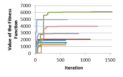 | Figure 9. 10 solutions without our pheromone function |
The final averaged quality in Figure 10 is much higher than the one in Figure 9. Furthermore, after 200 loops only a few better qualities were found (c.f. Figure 9), whether in Figure 10 after 3000 loops still much better qualities were found. In fact, the optimization takes longer to be finished (higher number of loops) but for getting a much better solution this is an acceptable effort of time.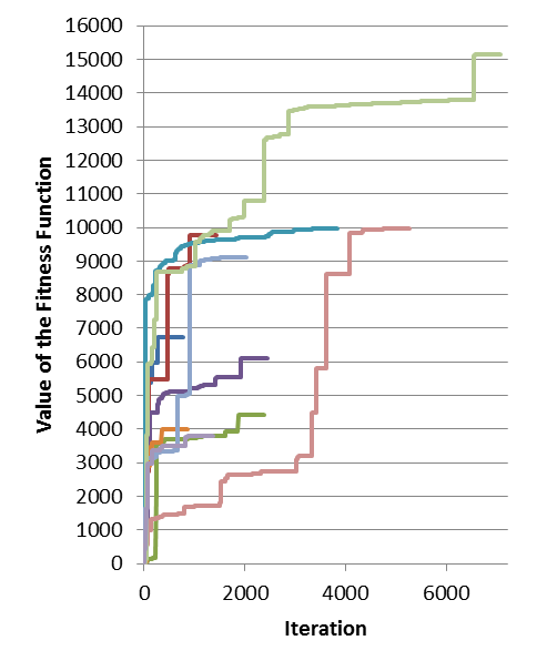 | Figure 10. 10 solutions with our pheromone function |
3.4. Sequence of the Algorithm
The algorithm can be divided into 8 steps, c.f. Figure 11. In Step 1, all variables will be initialized. This includes e.g. the maximum amount of loops without finding a better solution. This assures that the algorithm stops searching for a better solution after a defined amount of virtual ants are created regarding all the needed information for creating an allocation (the component, the initial pheromone values,...). All pheromone values have the same value at the beginning.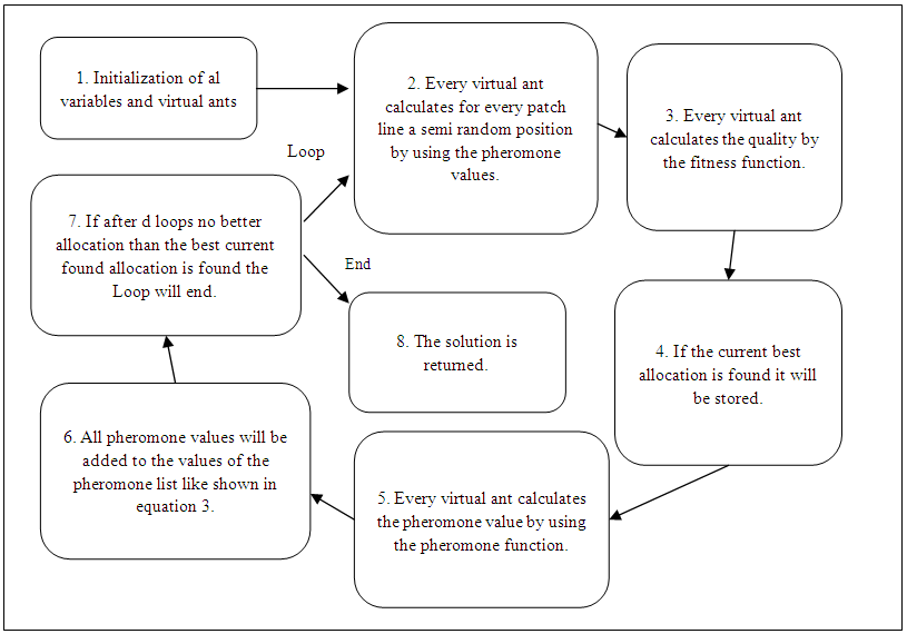 | Figure 11. The Algorithm Structure |
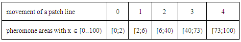
In Step 2, each virtual ant generates pheromone for every patch allocation. With increasing quality of this allocation, the pheromone value is increasing too. Those values are then transformed into areas. The size of these areas is represented by the quantity of the total pheromone value for this allocation.By generating a random number between 0 and total set of all values, an area and thereby an allocation is chosen. Table 2 for example shows a list of a patch line and its 5 movements. Movement 2 has an area of 34 (6-40) which is the highest area of all and therefore movement 2 has the highest possibility to be chosen. For example, the random search between 0 and 100 get the value 35 (c.f. Table 2). Regarding the table this values falls into the interval between 6 and 40. As result, movement 2 is chosen for this patch line. Before the first calculation, all pheromone values are equal, therefore the first allocation is completely generated by random. Table 2. Example of a Possible Pheromone Distribution of a Patch Line for Choosing the Next Movement
 |
| |
|
After generating one allocation for every virtual ant, every ant generates the quality by the fitness function (Step 3). If the quality value is the highest found until there, the value and the related allocation will be stored as the best allocation and the current solution (Step 4).In Step 5, the quality of each virtual ant is transformed to a pheromone value by the pheromone function and the pheromone values are adapted with that value in Step 6, c.f. Equation 3. The calculated values are only added to the pheromone values which movements have been chosen for the allocation. Therefore the formula has the value c=1 for a chosen movement and c=0 for all others. After that all past values Pi,j will be multiplied with a factor (1-e)<1 with e as the evaporation of the pheromone, c.f. equation 3, where the pheromone value Pi,j+1 corresponds to all the calculated values and g represent the value got from the pheromone function. The value i as a natural number refers to a moved patch line, n presents the number of the patch lines and s defines the number of discrete steps every patch line can move. Therefore, for every element i of a set of all moved patch lines the corresponding pheromone value will be adapted. The value j stands for the current loop and j+1 for the next loop.  | (3) |
To ensure that no pheromone value becomes zero, the formula lets all values aspire to the value 1, because if a value is zero the probability to choose the related movement is zero too. However, it cannot be excluded, that this movement is part of a solution. In the next step the algorithm checks whether the maximum amount of loops without finding a better allocation is reached. If the maximum value is reached the best found allocation will be returned in the last step, otherwise all virtual ants get new pheromone values and restart with finding a solution in Step 2.
3.5. Performance Optimization
For using that algorithm in practice, time is a very important factor. However, generating or moving a patch on a 3D surface cost a lot of time for calculating. Therefore, it is very time consuming to generate one allocation for every virtual ant in every loop.Since the patches are only moved in discrete steps, this allows caching moved patch lines in a list to reuse them if needed. After caching every possible allocation of a patch line there are no additional calculations of patch lines in 3D anymore necessary therefore the calculation is much faster: With increasing amount of loops the effect becomes more and more beneficial. Also all other used 3D calculations like for example the projection of a point in 3D for the fitness function could be cached. Therefore, in every loop no 3D calculations exist anymore which allows a practical use of this algorithm.
3.6. Influencing Factors of the Algorithm
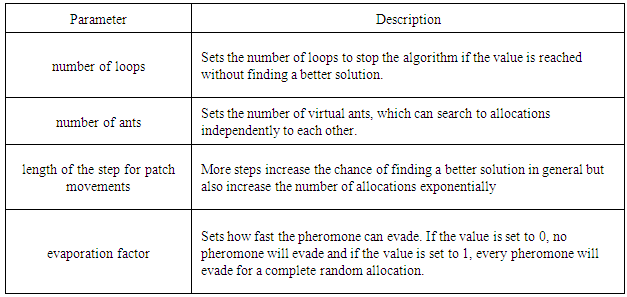
The following list contains parameters to influence the algorithm. For example to save calculation time, the number of loops can be reduced. However, this can reduce the quality of the found solution too.Table 3. Parameters to Configure the Algorithm
 |
| |
|
4. Applying of the Algorithm on an Example
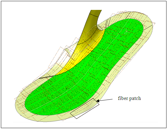
Analytic algorithms to find the best patch allocation need enormous calculation time. For example, a CAD model with 20 patch lines, 10 steps for every patch line and a calculation time of 1 millisecond for one solution takes 1020 milliseconds (about 3171 billion years) for finding the best solution. On the other hand, heuristic algorithm can also find suitable allocations for that kind of problems. The simplest algorithm for that is the random algorithm. To test that algorithm a medical orthosis imbedded in a closed CFK-tool chain is created, beginning with a CAD model over the patch allocation and simulation of the robot movements and finished by the manufacturing of a preform (c.f. Figure 12). The orthosis has a multi-curved surface and therefore high requirements for finding a good patch allocation. For the evaluation, only the complex sole of the foot is used for an optimized allocation (c.f. Figure 15).Figure 13 shows 10 optimizations using the random algorithm for the sole of the foot. Only one optimization generates a solution. For a use in practice, only one solution of 10 optimizations is not enough. Additionally if the component is getting more complex, the possibility to find solution with a random algorithm extremely decreases. The described algorithm can be located between these two previous described types of algorithms. It is much faster than analytic algorithm, as can be seen in Figure 14. After 10 optimizations, five are acceptable which is much better than the random algorithm illustrated in Figure 13. Therefore, our algorithm finds more and better solutions than a random function.That example shows that with this algorithm, for complex components a solution can be effectively generated. For example if the number of loops is set to a higher value, the possibility to find solutions will increase further.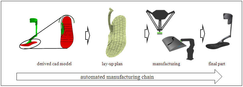 | Figure 12. Schematic manufacturing chain of an FPP component |
 | Figure 13. 10 solutions by a random algorithm |
 | Figure 14. 10 solutions by our algorithm |
 | Figure 15. Model of an optimized sole of a medical orthosis |
5. Conclusions
The presented FPP procedure is an automated manufacturing process for preforms with complex fiber architecture due to the high flexibility of the fiber orientation of the patches. Because fiber patches are used instead of endless fibers, the local fiber orientation can be adapted to the load of the component without restriction in radii. Due to the high amount of fiber patches for a preform the distribution of those patches has to be calculated automatically. Each position is affecting the mechanical properties of the final part. The patch allocation is realized by moving a group of patches to each other, which are lying on a patch line. Therefore an allocation exists where a special property criteria, in this case strength, reaches its maximum. This paper presents a procedure to allocate the patches automatically on a 3D-surface regarding a specific quality fitness function, which bases on experimental data. Because the patch lines can be moved independently from other patch lines, finding a good Solution is a NP problem. The heuristic algorithm, called ant colony algorithm used in this paper, is a good approach for solving such type of problems. The advantage can be shown by the presented example, a complex multi-curved structure. In that example, 5 of 10 optimizations create good solutions. That is five times more than a random search was achieving. Furthermore, all solutions of the developed procedure have a better quality than the one by random search. An important point of view is, that by increasing the amount of loops for finding a good solution the quality of the found solutions increase too. After finding a solution, the received position data for each patch can be used directly to calculate the necessary movement of the robot the manufacture the preform. In further research, the process chain will be developed further to get a better performance. A following step will be to adapt the algorithm to run in parallel to further increase its performance.
ACKNOWLEDGEMENTS
We acknowledge support by Deutsche Forschungsgemeinschaft and Open Access Publishing Fund of Clausthal University of Technology.
References
| [1] | R. Lässig, M. Eisenhut, A. Mathias, R. Schulte, F. Peters, T. Kühmann et al. Serienproduktion von hochfesten Faserverbundbauteilen: Perspektiven für den deutschen Maschinen- und Anlagenbau; 2012. |
| [2] | J. van Campen, C. Kassapoglou, Z. Gürdal. Generating realistic laminate fiber angle distributions for optimal variable stiffness laminates. Composites Part B: Engineering 2012;43(2):354–60. |
| [3] | C. S. Lopes, Z. Gürdal, P. P. Camanho. Variable-stiffness composite panels: Buckling and first-ply failure improvements over straight-fibre laminates. Computers & Structures 2008;86(9):897–907. |
| [4] | A. Khani, S. T. IJsselmuiden, M. M. Abdalla, Z. Gürdal. Design of variable stiffness panels for maximum strength using lamination parameters. Composites Part B: Engineering 2011;42(3):546–52. |
| [5] | M. Bannister. Challenges for composites into the next millennium — a reinforcement perspective. Composites Part A: Applied Science and Manufacturing 2001;32(7):901–10. |
| [6] | M. Lamontia. (Microsoft Word - SAMPE 2002 Lamontia Conformanble Compaction System Develop\205). |
| [7] | D. Lukaszewicz, C. Ward, K. Potter. The engineering aspects of automated prepreg layup: History, present and future. Composites Part B: Engineering 2012;43(3):997–1009. |
| [8] | A. W. Blom. Structural Performance of Fiber-Placed, Variable-Stiffness Composite Conical and Cylindrical Shells. Dissertation. Delft; 2010. |
| [9] | B. C. Kim. Limitations of Fibre Placement Techniques for Variable Angle Tow Composites and their process-induced Defects; 2011. |
| [10] | K. Götz. Die innere Optimierung der Bäume als Vorbild für technische Faserverbunde - eine lokale Approximation. Dissertation. Karlsruhe; 2000. |
| [11] | T. Rettenwander, M. Fischlschweiger, M. Machado, G. Steinbichler, Z. Major. Tailored patch placement on a base load carrying laminate: A computational structural optimisation with experimental validation. Composite Structures 2014;116:48–54. |
| [12] | M. R. Wisnom. On the Increase in Fracture Energy with Thickness in Delamination of Unidirectional Glass Fibre-Epoxy with Cut Central Plies. Journal of Reinforced Plastics and Composites 1992;11(8):897–909. |
| [13] | O. Meyer. Kurzfaser-Preform-Technologie zur kraftflussgerechten Herstellung von Faserverbundbauteilen. Dissertation. Stuttgart; 2008. |
| [14] | K. Singh, K. Kurbel. Ease-of-use, implementation and performance of heuristics for optimization – A comparison of evolutionary and iterative improvement methods. International Journal on Artificial Intelligence Tools 2001(10):S. 407–419. |
| [15] | M. Dorigo, M. Birattari. Ant colony optimization. Encyclopedia of Machine Learning 2010:36–9. |
| [16] | M. Dorigo, L. M. Gambardella. Ant colony system: a cooperative learning approach to the traveling salesman problem. IEEE Transactions on Evolutionary Computation 1997(1/1):417–23. |
| [17] | Y. C. Liang, A. E. Smith. An ant colony optimization algorithm for the redundancy allocation problem (RAP). IEEE Transactions on Reliability 2004(53/3):417–23. |
| [18] | L. M. Gambardella, E. D. Taillard, M. Dorigo. Ant colonies for the quadratic assignment problem. Journal of the operational research society 1999:167–76. |
| [19] | S. Lin, B. W. Kernighan. An effective heuristic algorithm for the traveling-salesman problem. Operations research (21/2): 498–516. |
 Abstract
 Reference
 Full-Text PDF
 Full-text HTML