1. Introduction

If the results on modeling of the behavior of composite materials are well established using the homogenization theory of periodic media [1], certain situations, as this paper shows, deserve to rethink completely the modeling approach [2] [3]. Indeed, by considering a laminated composite structure in which was developed a damage by debonding, we show that the behavior of such structure is not that of a simple material, where the results are classical and well known [4] [5] [6], but that of a micro-structured media: one must add to the classical macroscopic displacement field, a field of planar vectors, representing the relative sliding of stiff layers with respect to the soft ones. And consequently, new homogenized tensors and new coupled equilibrium equations appear [2] [3]. It is the purpose of this paper.

Specifically, the paper is organized as follows. The next section is devoted to the setting of the problem: one consider a laminated composite structure, occupying the open bounded domain of IR3 constituted by a periodic distribution of stiff elastic layers embedded and stacked in the direction e3(see Figure 1) in an elastic matrix(soft layers). In a part noted the stiff layers are assumed perfectly bonded to the matrix while in the complementary part noted they are assumed to be debonded but still in contact without friction with the matrix. The number of folds n is assumed large enough (so that the microstructure parameter 1/n is small enough [1] [7] [8] [9] [10] [11]). The problem consist in finding the displacement field and the associated stress field (limits respectively of when n goes to infinity) solutions of the real problem (1)-(4) which can be written in variational form (5)-(7). The third section is devoted to a brief review of the homogenization theory of periodic media and the writing of equations governing the fields (three first terms of asymptotic expansion of [3]) whose goal to determine the displacement field limit The fourth section is divided into three sub-sections. The sub-section 4.1 is devoted to the determination of the form of the displacement field This displacement form is given by the expression (15) which valid in the two part 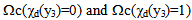[2] [3]. In this last part we remark the appearance of a new macroscopic field (noted forgotten in the existent literature (see [4] [12] [13] [14] [15] and [16] [17] [18] [19] [20]), interpreted as the relative sliding between the stiff and soft layers [3]. This is due to the fact that the layers considered, in the part are completely debonded. In sub-section 4.2, we simply explicit the variational equations, capable to express in terms of We obtain the classical ones in given by (20), and other ones in given by (27). 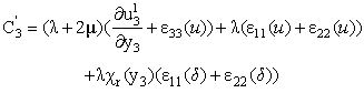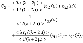The equations obtained in contain additional terms that dependent of the derivatives of with respect to the macroscopical coordinates x1, x2 and x3. The sub-section 4.3 is devoted to the writing of the homogenized problem. Exploiting the form of displacement field given by (15) and the integral equations, linking the fields given by (21)-(23) and (28)-(30), we determine the macroscopic problem governing the displacement field This problem is given in variational form by (47) or distribution form by (48). 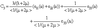We will remark the appearance of new homogenized tensors which are interpreted respectively as the stiffness tensor to the relative deformation of debonded folds(stiff and soft) and the tensor of internal stresses generated in the cell by an extension of these folds. And we finally conclude in the last section.

2. Position of the Problem and Notations

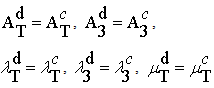
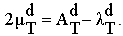
We work in the framework of linear elasticity and we consider a laminated composite structure whose natural reference configuration is the open bounded domain of IR³ with a smooth boundary We denote by (e₁, e₂, e₃) the canonical basis of IR³ and (x₁, x₂, x₃) the coordinates of a point x of . The structure is assumed constituted by two materials: stiff layers qualified of reinforcing and soft layers(matrix) playing the role of binder. The two constituents of the composite structure are assumed elastics, homogeneous and isotropic whose Lamé coefficients are The number of folds n is assumed large enough for that the period of the microstructure 1/n is small enough. In a part the stiff layers are assumed perfectly bonded to the matrix while in the complementary part they are assumed debonded but still in contact with the matrix. The structure is assumed submitted to an external loading applied on the boundary Specifically, we fix a part and we apply a surface force density F on the complementary part of boundary (see Figure 1). The body force density is assumed negligible.

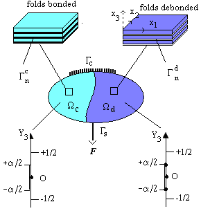Figure 1. The laminated composite and the two unite cells Y and Y\

We assume that in the part and during the deformation, the stiff layers remain in contact with the matrix and can slip without friction. This expresses then that the normal displacement field is continuous and the shear vanish on the debonded interfaces of the part by cons, the displacement and the stress fields are continuous on the bonded interfaces Denoting by A(x) the linearized elasticity tensor into a point x, the divergence and the symmetrized gradient with respect to x, the real elastic problem consists in seeking for the couple checking the following static equilibrium equations:

(1)

(2)

(3)

(4)

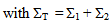
where the last line translates the continuity of normal displacement field the continuity of the stress vector and the nullity of the shear on the debonded interfaces This problem is written in distribution form. We can write it in variational form: it consists in finding such that

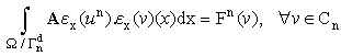(5)

with

(6)

(7)

3. Application of Homogenization Theory

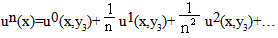
Following the classical two-scale procedure in homogenization theory of periodic media [3] [4], we assume that uⁿ can be expanded as follows:

(8)

where y₃=nx₃ is the microscopic variable, describing the cell according to x is in with Y=[1/2,+1/2] and denotes the volume fraction of the stiff folds into the matrix). And the uⁱ=(uⁱ₁, uⁱ₂, uⁱ₃), are the Y-periodic fields with respect to the variable microscopic y₃.

By substituting the development postulated (8) of uⁿ into the variational problem (5) and by identifying formally the terms of same power of n, we obtain a sequence of interrelated problems whose the unknowns are the fields uⁱ(x,y₃), The determination of the first term u⁰(x,y₃) in the asymptotic expansion of uⁿ(x) provides the effective behavior sought of the microstructure We write thus only the three first problems of order, n², n¹ and n⁰. And this sufficient for the determination of u⁰.

(i) At order n²:

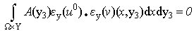(9)

(ii) At order n¹:

(10)

(iii) At order n⁰:

(11)

where

(12)

Remark: The integrals on must be understood as the sum of integrals on

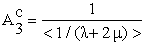
4. Resolution and Asymptotic Results

4.1. Form of the Displacement Field u⁰

The equation (9) allows having the form of the unknown displacement field u⁰. Indeed, by choosing as function test v(x,y₃)=u⁰(x,y₃) in the equation (9) and owing the positivity of the elasticity tensor A, we deduce that the microscopic strain tensor of u⁰ vanish, i.e. in Y or in according to x is in Therefore u⁰, considered as function of y₃, is a rigid displacement. Therefore

● The rigid displacements of the cell Y, associated at the bonded part are translations because Y is a connected part of IR. We find the classical and known result:

(13)

u being the classical displacement field in the homogenization theory of periodic media.

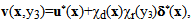
● The rigid displacements of the cell associated at the debonded part are also translations, but since is the union of two connected parts Y_m and Y_r, each part has its own translation. So, we get a relative translation of Y_r compared to Y_m. And the displacement field u⁰ can be written then, for as follow:

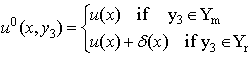(14)

with

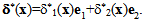
It should be noted that we find once again the classical displacement field u which interpreted as displacement field of the matrix. By cons there is birth of a new field forgotten in the existent literature [12] [13] [14] [15]. It modeling the relative sliding of stiff layers with respect to the soft ones.

Remark: We can have a single expression (instead of two (13) and (14)) of the displacement field u⁰ valid in defined as follow:

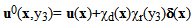(15)

where are the characteristic functions, associated respectively to defined by:

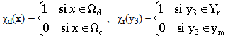(16)

The macroscopic strain field associated to the displacement u⁰ is then given by:

(17)

where denotes the strain tensor of the sliding field given by:

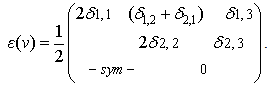(18)

We agreed here the simplistic notation as derivative of the scalar field with respect to

4.2. Expression of u¹ in Term of u⁰

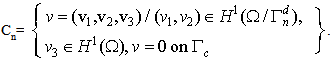
Assuming for the moment that the fields u and are known, the equation (10), connecting u¹ to u^0, will allow us to determine u¹ in terms of the gradient of u and . Indeed, taking into account (15) and coefficients of the elasticity tensor given by

(19)

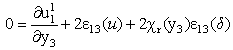
(where denote the Kronecker symbol equal to 1 if i=j and 0 otherwise) and by choosing functions tests well defined, of the form we can express u1(x,y3), in terms of u and . In always distinguishing we obtain:

(i) In the equation (10) becomes:

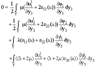(20)

This is obtained in choosing with is the space of infinitely differentiable functions with compact support in We then deduce from (20) that

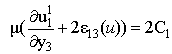(21)

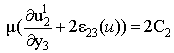(22)

(23)

where C₁, C₂ and C₃ are constants with respect to y₃ and well defined. Indeed, denoting by the mean value of f over the cell Y we get, since (because of the Y-periodicity):

(24)

(25)

(26)

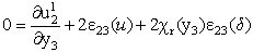
(ii) In we obtain, in the same manner, a variational equation which is valid for any Y-periodic field verifying

(27)

from which we deduce that(because of the possibility of a tangential discontinuity of the displacement and the nullity of the shear):

(28)

(29)

(30)

where C'₃ is given by ( since )

(31)

5. Macroscopic Homogenized Problem

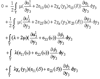
From the equations (9) and (10) we found the form of displacement field u⁰ in terms of u and (given by (15)) and we obtained equations connecting this fields to u¹ (given by (21)-(23) and (28)-(30)). Now, using equation (11), we should obtain a variational equation governing only the fields u and . Let consider for that, a particular test field v(x, y₃) verifying

(32)

with The equation (11) is simplified and the displacement of order 2, disappear in this equation and we can write it:

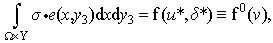(33)

with

(34)

where we have posed,

(35)

and

(36)

Multiply these two last expressions of tensors and integrating the result obtained over the cell Y, taking into account the relations connecting u¹ to u and (given by (21)-(23) in and (28)-(30) in we obtain, in distinguishing always and the following results:

(i) In

(37)

denotes the homogenized stiffness tensor of the bonded laminated composite part. The macroscopic relation stress-strain is given by the following matrix representation:

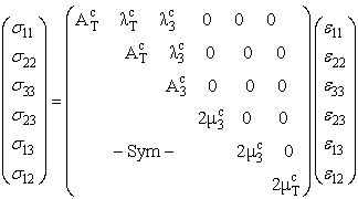(38)

with,

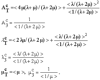(39)

where

Five coefficients are independent in the expression of tensor , the homogenized structure is thus transversely isotropic.

(ii) In

After some simplifications which we give not the details here(you can see the details in [3]), we get:

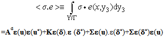(40)

where,

● denotes the homogenized stiffness tensor of the debonded laminated part, but without deformation of the stiff layers, given by

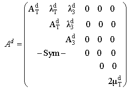(41)

with,

(42)

with,

Four independent coefficients only, the terms A^d₁₃₁₃ and A^d₂₃₂₃ are null because of the nullity of shear on the debonded interfaces. The homogenized structure obtained is also transversely isotropic.

● K is interpreted as the rigidity tensor to the relative plane deformation of the debonded stiff layers (but in contact with the matrix). It is given by

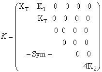(43)

with,

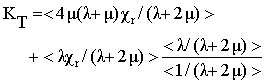
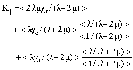(44)

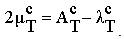
with K_T = K₁ + 2K₂

● is interpreted as the stress tensor resulting of internal stresses generated in the cell by an internal extension of the debonded stiff layers (but in contact with the matrix). It is given by

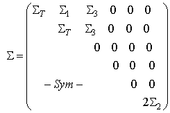(45)

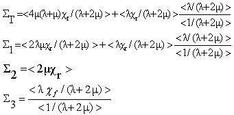
(46)

Remark: One can show that the tensors, A^c and A^d, are symmetric and definite positive. And A^c is greater than A^d in sense of quadratic forms [3] [21]. K is also symmetric. by cons is not symmetrical: as operator, it acts on two types of spaces of test functions, associated at fields u and [3].

From (33), (37) and (40), we obtain finally that the macroscopic displacement fields u and are solutions of the following variational effective problem:

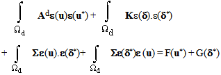(47)

for all displacement fields, kinematically admissible.

Remark: The expressions of show that only the derivatives, with respect to x_ and x₂, of sliding appear in the variational formulation (47). is thus seeking for in a space of functions f=(f₁,f₂) square integrable over and whose only the derivatives square integrable on But this pose problem of verification of the boundary conditions, since such fields does not admit necessarily a trace on the boundary. In fact, we can define f at a point x of a surface provided that the components n₁ or n₂ of the normal n of at this point is nonzero. Thus we will write on and on One must note also that there is a coupling, via the stress tensor between the displacement field of stiff layers and the displacement field of the matrix u.

Let us write now the homogenized problem which deduced from the variational problem (47) above. It consists to finding a displacement field u and a stress field such that

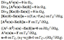(48)

The three first equilibrium equations must be understood in the sense of distributions when the loading is not sufficiently smooth. The two first ones are three-dimensional equations valid respectively in while the third one is a bidimensional equations family of plane type, indexed by representing the normal force). We see that in the second equation the term play the role of a pre-stressed field of the medium, while in the third equation, the term play the role of a pre-stressed field of a planar medium. This system of equations is completed by boundary conditions that we deduce also from (47).

6. Conclusions

The three-dimensional study made on the effective behavior of a laminated composite material, whose stiff folds are perfectly bonded to the matrix in a part of this structure and debonded in the complementary part but still in contact with the matrix, shows that:

● In the perfectly bonded part, the results obtained are the classical properties of homogenization theory which stands that the leading term of the asymptotic displacement field expansion given by (13) does not depend on the microscopic coordinates, and in the homogenized problem appear the classical homogenized stiffness tensor given by (38)(39). However, these properties hold true only when the folds are perfectly bonded to the matrix.

● By cons in the debonded complementary part, the result obtained differs from the usual property of the homogenization theory. Indeed, because of debonding of the stiff folds from the matrix, the leading term of the asymptotic displacement field expansion depends here on the microscopic coordinates. Moreover a new macroscopic vector field enters in the effective kinematic of the laminated composite. Specifically, we obtain a classical vector field representing the macroscopic displacement of the matrix and an additional vector field representing the relative slip of the stiff layers with respect to the matrix given by (14). And the homogenized problem (48) obtained is not classic. It contains new homogenized tensors coupling those two vector fields, given by (43)(44) and (45)(46), ignored in the existent literature.

We finally conclude that, the effective behavior of a laminated composite material in the case where the folds are debonded but still in contact with the matrix is formally similar to a generalized continuous medium whose kinematics is not described only by the usual macroscopic displacement field but also a other displacement field describing the sliding of the stiff layers.