1. Introduction

The catalytic membrane reactor as a promising novel technology is widely recommended for carrying out heterogeneous reactions. A number of reactions have been investigated by means of this process, such as dehydrogenation of alkanes to alkenes, partial oxidation reactions using inorganic or organic peroxides, as well as partial hydrogenations, hydration, etc. As catalytic membrane reactors for these reactions, intrinsically catalytic membranes can be used (e.g. zeolite or metallic membranes) or membranes that have been made catalytic by dispersion or impregnation of catalytically active particles such as metallic complexes, metallic clusters or activated carbon, zeolite particles, etc. throughout dense polymeric- or inorganic membrane layers[1]. In the majority of the above experiments, the reactants are separated from each other by the catalytic membrane layer. In this case the reactants are absorbed into the catalytic membrane matrix and then transported by diffusion (and convection) from the membrane interface into catalyst particles where they react. Mass transport limitation can be experienced with this method, which can also reduce selectivity. The application of a sweep gas on the permeate side dilutes the permeating component, thus increasing the chemical reaction gradient and the driving force for permeation (e.g. see Westermann and Melin[2]). At the present time, the use of a flow-through catalytic membrane layer is recommended more frequently for catalytic reactions[2]. If the reactant mixture is forced to flow through the pores of a membrane which has been impregnated with catalyst, the intensive contact allows for high catalytic activity with negligible diffusive mass transport resistance. By means of convective flow the desired concentration level of reactants can be maintained and side reactions can often be avoided (see review by Julbe et al.[3]). When describing catalytic processes in a membrane reactor, therefore, the effect of convective flow should also be taken into account. Yamada et al.[4] reported isomerization of 1-butene as the first application of a catalytic membrane as a flow-through reactor. This method has been used for a number of gas-phase and liquid-phase catalytic reactions such as VOC decomposition[5], photocatalytic oxidation[6], partial oxidation[7], partial hydrogenation[8-10] and hydrogenation of nitrate in water[11].

From a chemical engineering point of view, it is important to predict the mass transfer rate of the reactant entering the membrane layer from the upstream phase, and also to predict the downstream mass transfer rate on the permeate side of the catalytic membrane as a function of the physico-chemical parameters. If this transfer (permeation) rate is known as a function of the reaction rate constant, it can be substituted into the boundary conditions of the differential mass balance equations for the upstream and/or the downstream phases. Basically, in order to describe the mass transfer rate, a heterogeneous model can be used for larger particles and/or a pseudo-homogeneous one for very fine catalyst particles[12]. Both approaches, namely the heterogeneous model for larger catalyst particles and the homogeneous one for submicron particles, have been applied for mass transfer through a catalytic membrane layer. Nagy[12] has analysed diffusive mass transport through a membrane layer with dispersed catalyst particles. It was shown that both the heterogeneous and the pseudo-homogeneous models give practically the same results in the very fine, sub-micrometer particle size range. The convective velocity was not taken into account in Nagy’s model[12] cited. Recently Nagy analysis the effect of the convective velocity on the enzyme catalysed reaction[13] as well as summarizes the most important mass transport equations of a membrane layer taking also into account the simultaneous effect of the convective and diffusive flows[14,15]. These papers extend previous investigations by including the effect of convective flow, applying two different operating modes, namely with and without sweep phase on the permeate side as well as two different models, namely an approaching and the exact models. Mathematical equations have been developed to describe the simultaneous effect of diffusive flow and convective flow and this paper analyses mass transport and concentration distribution by applying the model developed. The pseudo-homogeneous model will be presented in detail, assuming that the catalyst particles are in the nanometer-sized range, as this is the case in most catalytic membrane reactors.

The main purpose of this paper is to present the various steps of the mathematical solutions, as well as to study the effect of mass transport parameters of the catalytic membrane layer on the mass transfer rates. At the end of this paper, the predicted data are compared with measured ones taken from the literature. The method presented in this paper can also be applied to higher order chemical reactions.

2. Theory

In this section different mathematical models will be shown and solved in order to describe the mass transport through catalytic membrane layer with forced flow through it. It is assumed that the catalyst particles are very fine particles with size less than 1 μm. Thus, the so called pseudo-homogeneous model[12,14,15] was applied for description of the mass transport through the catalytic membrane layer. The catalyst particle can be porous one (e.g. zeolite particles), or dense one without diffusivity inside it (e.g. metal clusters). Accordingly, different mass transfer rate equations can be defined between the membrane and particles as will be shown in this section.

In order to increase the efficiency of the catalytic membrane, the size of particles chosen should be as low as possible[12]. The use of nanometer-sized catalyst particles is thus recommended. The differential mass balance equation for diffusive and convective flows in the catalytic membrane layer, for unsteady-state, can be as:

(1)

with initial and boundary conditions as:

if t = 0, y > 0 then C=C^o

if t > 0, y = 0 then C=C^*

if t > 0, y = δ then C=C^o

The functions Q provides the specific source term induced by the mass transport into the catalytic nanoparticles distributed uniformly in the catalytic membrane layer. The mass transfer rate into the catalytic particle can depend on the external mass transfer resistance around the particles as well as on the internal transport accompanied by chemical reaction. Note that in the case of nanometer-sized particles the diffusion time, t_D, (t_D=R²/D_p) can be very small, thus, it can easily be much shorter than the reaction time, t_r (t_r=1/k₁ for first-order reaction). This fact should be taken into account to define the Q value. E.g. for d_p=100 nm and D_p=1 x10^-12 m²/s, the diffusion time is equal to 0.01 s. In the slow reaction rate regime, if , the saturated concentration, C^*, can exist throughout the particle, i.e. if t_r < 9 s according to the above example. In this case the so called effectiveness factor is considered to be unit and accordingly the internal mass transport can be regarded to be instantaneous.

2.1. Mass Transport into the Dispersed Nanometer-Sized Catalyst Particles

Two important cases will be discussed, namely instantaneous and finite internal mass transport rates. Both cases can be important when chemical reaction takes place inside of the particles or on the particle surface. As chemical reaction, the first-order one will be discussed. Several non-linear reactions can be approached by first-order one dividing the membrane layer into thin sub-layers as will be shown in the Appendix. Accordingly these reactions can be handled as first-order ones.

2.1.1. Mass Transport Rates with Instantaneous Internal Mass Transport

The chemical reaction takes place on the internal interface of the catalyst particles with the reaction rate: where is the reaction rate constant related to the catalyst interface, m³/(m²s), is the available catalytic surface area per unit volume of catalyst, m²/m³, and k₁ also rate constant, 1/s (). Thus, one can obtain applying the known Henry equation for the catalyst interface, namely HC= as:

(2)

In Eq. (2) the external mass transfer resistance is neglected, thus the interface concentration of the catalytic particles is equal to the “bulk” one in the membrane matrix.

In the case of inorganic catalyst particles, as zeolite, the Langmuir-Hinshelwood kinetics the most commonly used kinetic expression to explain the heterogeneous catalytic process[16]. Assuming that the reaction of a component occurs in a simple unimolecular elementary reaction step and that the kinetics are first order with respect to the surface concentration of the adsorbed reactant, the reaction rate can be expressed as[16]:

(3a)

This reaction is often approximated to first-order kinetics for condition KC << 1 or to zero-order kinetics for condition KC >> 1. Similar kinetic expression can be applied for biochemical reactions according to the Michaelis-Menten or Monod kinetics:

(3b)

Replacing Eqs. (3) into Eq. (1), the differential equation obtained for steady-state case can only be solved by analytical approach (this will be shown in Appendix) or numerically. How the Eqs. (3) can be linearized is given by Eq. (A1) in the APPENDIX.

2.1.2. Mass Transport with Finite Internal Mass Transport

It the reaction rate is fast then there can be strong concentration gradient inside of the particle, thus the internal transport should also be taken into account. The internal specific mass transfer rate in spherical particles, J_p, for steady-state conditions and when mass transport is accompanied by a first-order chemical reaction, can be given according to Bird et al.[17] as follows:

(4)

where

(5)

and

The external mass transfer resistance through the catalyst particle depends on the thickness of the diffusion boundary layer, δ_p. The value of δ_p can be estimated from the distance between particles[12]. As this value is limited by neighboring particles, the value of β_p will be somewhat higher than that calculated from the well known equation, namely 2 = β_pd_p / D_p, where the value of δ_p is assumed to be infinite. This results in:

(6)

where

From Eqs. (5) and (6), for the mass transfer rate with overall mass transfer resistance with H_p = C_p/C:

(7)

Thus, the value of Q will be as:

(8)

where ω is the catalyst surface per membrane volume, m²/m³

2.1.3. Reaction Occurs on the Outer Interface of the Catalytic Particles

It often might occur that the chemical reaction takes place on the interface of the particles, e.g. in cases of metallic clusters, the diffusion inside the dense particles are negligibly. Assuming the Henry’s sorption isotherm of the reacting component onto the spherical catalytic surface (CH_f = q_f), applying DdC/dr = k_fH_fC boundary condition at the catalyst’s interface, at r = R, the Φ reaction modulus can be given for first-order reaction, as follows[see Eq. (11) for Φ]:

(9)

where

(10)

where k_f is the interface reaction rate constant. The above model is obviously a simplified one.

2.2. Mass Transport in the Catalytic Membrane Layer

Taking into account Eqs. (2) or (8) as source term, one can get simple first-order kinetics. The differential mass balance equation for the polymeric or macroporous ceramic catalytic membrane layer, for steady-state, taking both diffusive and convective flow into account, can be given, according to Eq. (1), as:

(11)

where

; ;or

where υ denotes the convective velocity, D is the diffusion coefficient of the membrane, and δ is the membrane thickness. The membrane concentration, C is given here in a unit of measure of gmol/m³. This can be easily obtained by means of the usually applied in the e.g. g/g unit of measure with the equation of C = wρ/M, where w concentration in kg/kg, ρ – membrane density, kg/m³, M-molar weight, kg/mol.

(12)

Introducing a new variable, [see Eq. (12)] the following differential equation is obtained from Eq. (11):

(13)

where

The general solution of Eq. (13) is well known[14], so the concentration distribution in the catalytic membrane layer can be given as follows:

(14)

with

The inlet and the outlet mass transfer rate can easily be expressed by means of Eq. (14). The overall inlet mass transfer rate, namely the sum of the diffusive and convective mass transfer rates, is given by:

(15)

The outlet mass transfer rate is obtained in a similar way to Eq. (15) for Y=1:

(16)

The value of parameters T and S can be determined from the boundary conditions which can vary according to the operating conditions used. Assuming that the external mass transfer resistance on the feed side, namely the diffusive resistance, is not negligible, the simultaneous effect of the fluid boundary layer should also be taken into account. Basically, the effect of the external, diffusive mass transfer resistance, in presence of convective flow can be described by two models: (i) the diffusive mass flow is regarded to be constant through the boundary layer (this diffusive flow is called as Fickian one in this paper), accordingly the sum of the diffusive and convective flows varies in the boundary layer (Model A) or (ii) that it varies in the boundary layer, according to the change of the convective mass flow due to the curvature of the concentration in the boundary layer (Model B). This latter one should be regarded as exact solution, namely the sum of the diffusive and convective flows is constant throughout the boundary layer. According to the mass transfer conditions of the permeate phase, namely there is a sweep phase or there is not sweep phase, two operating modes will be distinguished according to Figs. 1a and 1b.

Figure 1. Concentration distribution in the membrane reactor with convective flow applying a sweep phase on the permeation side (Fig. 1a) and without sweep phase (Fig. 1b)

The essential difference between the models is that there is a sweep phase that can remove the transported component from the downstream side providing the low concentration of the reacted component and its high diffusive mass transfer rate (dC/dY > 0; Models A₁ and B₁). There is no sweep phase, thus the outlet phase is moving by convective flow from the membrane due to the lower pressure on the permeate side and there is no diffusive flow, on the outlet membrane interface (dC/dY = 0; Models A₂ and B₂).

2.2.1. Mass Transport Models with Fickian Diffusive Flow in the Boundary Layer (Approaching Solution, Models A)

The simultaneous effect of the membrane and the boundary layers, on the mass transport, is taken into account. In presence of the convective flow, the overall mass transfer rate will be the sum of the diffusive and convective flows. Regarding the effect of the boundary layers on both sides of the membrane, the boundary conditions can be different on the feed side and permeate side, depending on the operating mode. Note that the Fickian diffusive flow along the diffusion path[as it is given in Eqs. (17) and (18)] assumed that the concentration distribution is linear, the concentration gradient is constant, in the boundary layer, independently of the presence of convective flow. Accordingly, the sum of the diffusive and the convective flow will change throughout the boundary layer due to the concentration change. In the reality, the concentration curve will be concave one due to the convective velocity thus, the sum of the diffusive and the convective flow remains constant as a function of the local coordinate in the boundary layer.

Model A₁ (dC/dY>0 at Y=1). In this case, due to the effect of the sweeping phase, the external mass transfer resistance on both sides of the membrane should be taken into account in the boundary conditions, though the role of is gradually diminished as the catalytic reaction rate increases. The concentration distribution in the catalytic membrane, when applying a sweep phase on the two sides of the membrane, is illustrated in Figure 1a. On the upper part of the catalytic membrane layer, in Fig. 1a, the fine catalyst particles are illustrated with black dots. It is assumed that these particles are homogeneously distributed in the membrane matrix. Due to sweeping phase, the concentration of the bulk phase on the permeate side may be lower than that on the membrane interface. The value of here denotes the liquid or gas phase concentration on the bulk phases (see Fig. A1), on both sides of the catalytic membrane layer. The boundary conditions can be given for that case as:

(17)

(18)

Boundary conditions given by Eqs. (17) and (18) are only valid in two phase flows. Where and denotes the interface concentration on the both sides of membrane layer, and are mass transfer coefficients in the continuous phase, β^o the membrane mass transfer coefficient (β^o = D/δ), H denotes the distribution coefficient between the continuous phase and the membrane phase. The solution of the algebraic equations obtained, applying Eqs. (14) to (18) can be received by means of known mathematical manipulations. Thus, the values of T and S obtained are as follows:

(19)

and

(20)

where

; ;

; ;

An important limiting case should also be mentioned, namely the case when the external diffusive mass transfer resistances on both sides of membrane can be neglected, i.e. when and . For that case the concentration distribution and the inlet mass transfer rate can be expressed by Eqs. (21) and (22), respectively[14].

(21)

(22)

with

(23)

Model A₂ (dC/dY=0 at Y=1). For the convective flow catalytic membrane reactor operating in another mode, for instance in dead-end mode as in Figure 1b, the boundary condition on the permeate side of the membrane should be changed. In this case the concentration of the permeate phase does not change during its transport from the outer membrane interface, and consequently dC/dY = 0. If there is no sweeping phase on the downstream side then the correct boundary conditions will be as[the value of J is defined by Eq. (15)]:

(24)

(25)

After solution one can get as:

(26)

(27)

2.2.2. Models with constant diffusive plus convective flows in the boundary layer (exact solution, Models B)

This, so called exact, model takes into account that the concentration change is not linear due to the presence of the convective flow but the sum of the convective and the diffusive flows will be constant throughout the boundary layer. The differential mass balance equation, given for the boundary layer, should be solved. That is, with constant transport parameters and in dimensionless space coordinate as (Y=y/δ₁, δ₁ is the thickness of the feed boundary layer, m):

(28)

where (Pe_L1 denotes the Peclet number in the boundary layer)

The solution of differential equation, Eq. (28) is as follows[14]:

(29)

Values of T and S parameters can be determined, without external diffusive mass transfer resistances, by the boundary conditions as:

(30)

(31)

The concentration distribution, applying Eqs. (30) and (31) as boundary conditions, is as follows:

(32)

Thus, the physical mass transfer rate, through the boundary layer, can be obtained, by means of Eq. (33), taking into account both the diffusive and the convective flows[see Eq. (15)] as follows:

(33)

where

(34)

Note that the physical mass transfer coefficient in the case of the simultaneous effect of the diffusion and convection,

, (denotes the overall mass transfer coefficient in presence of convective plus diffusive flows) can be much higher than that of the diffusive mass transfer coefficient, . The value increases linearly if Pe_L1 > about 3. It is also to be noted that the driving force depends on the Peclet number as it is given by Eq. (33). With the increase of the Pe_L1-number, the driving force also increases. In limiting case, namely if Pe_L1→∞, the value of . Note that if the diffusive flow is equal to zero on the down stream side of the boundary layer then the mass transfer rate on the down stream side is as: J = υ, thus this fact does not automatically mean that the outlet concentration gradient is equal to zero.

Knowing the mass transfer rate into the boundary layer (Eq. 33) and the membrane layer[Eq. (22) for Model A1 and Eq. (39) for Model B₁], applying the well-known resistance-in-series model, the overall mass transfer rate can be given for the above case, as well.

Model B₁ (dC/dY>0 at Y=1): The overall inlet mass transfer rate, applying Eqs. (22) and (33) is, for first-order chemical reaction in the membrane layer, as follows:

(35)

where

(36)

and

(37)

The value of β is defined by Eq. (23). Note that the mass transfer resistance in the boundary layer of the permeate side is not involved in Eq. (35). It can be given, but that case is not discussed here because its complexity and of its lesser importance due to the chemical reaction.

Model B₂ (dC/dY=0 at Y=1). Look at first the concentration distribution and the mass transfer rate in the membrane layer for that case, namely when dC/dY = 0 at Y=1. Assuming that there is no mass transfer resistance in the feed phase, thus, at Y=0 then , Applying to it Eq.

(25) as boundary condition for the permeate side, and using Eq. (14), one can get as[13]:

(38)

with Φ and Θ defined after Eqs. (11) and (13). Note that Eq. (38) does not involve the external mass transfer resistances. The inlet mass transfer rate, namely the sum of the diffusive and the convective flows, can be given as:

(39)

The overall mass transfer rate, applying Eqs. (33) and (39), will be as:

(40)

with

(41)

where and β is defined by Eqs. (34) and (39).

2.3. Intrinsically Catalytic Membrane Reactor

In this case, only the value of Ф differs from that of the catalytic membrane layer with dispersed catalyst particles. In the case of a first-order reaction, the value of Ф can be expressed for an intrinsic membrane layer with the following simple equation:

(42)

The mass transfer rate or the concentration profile can be estimated in a similar way to that for a membrane layer with dispersed catalyst particles. This case is not discussed in detail in this paper. The effect on the mass transfer rate and concentration distribution in the membrane reactor is basically the same as that obtained by the model developed for dispersed catalyst particles.

3. Results and Discussion

Two important transport models for convection flow catalytic membrane layer are presented in this paper. The difference between them is determined by the flow conditions on the permeate side, namely the permeated component is transported by a sweep phase from the membrane interface (dC/dY>0 at Y=1, Models A₁ and B₁) or there is no sweep phase (dC/dY=0 at Y=1, Models A₂ and B₂) on the permeate side. Obviously, these models can give essentially different inlet mass transfer rate. On the other hand, two important cases are also discussed regarding the external mass transfer resistance, namely modeled it by the so called Fickian diffusion flow (Models A₁ and A₂) and by the so called exact model, where the diffusion flow permanently increases due to the decreasing convective flow (their sum should be constant throughout the boundary layer) on the diffusion path in the boundary layer (Models B₁ and B₂).

3.1. Models for Membrane Reactor with Sweep Phase on the Permeate Side (dC/dY>0 at Y=1)

Figure 2. Concentration distribution in the membrane layer at different values of the reaction modulus, Φ, applying the Fickian diffusion flow in the boundary layers (Model A1 dC/dY>0 at Y=1); ( m/s; ; Pe=1; PeL1=1; []; H=1; )

Note that the application of the Fickian diffusion flow for the inlet and the outlet boundary layers[Eqs. (17) and (18)] is an approximation. The question is that its application can be acceptable and under what conditions. Typical concentration distribution curves of a catalytic membrane layer are shown for Model A₁ (Fig. 2) and for Model B₁ (Fig. 3).

The concentration was predicted by Eqs. (19) and (20) as well as by Eq. (21).

Figure 3. Concentration distribution in the membrane layer at different values of the reaction modulus, Φ, applying the exact diffusion flow in the inlet boundary layers (Model B1 dC/dY>0 at Y=1); ( m/s; ; Pe=1; PeL1=1;[ ]; H=1; )

The value of , (see Fig. A1) in Eq. (21), was predicted by means of Eq. (33) knowing the J value from Eq. (22). As you know there is a sweep phase on the permeate site, consequently there is a diffusive flow, as well on the outlet membrane interface, in both cases. The transport parameters were chosen to be the same for both models (m/; Pe=1; Pe_L1=1; , thus, the ν convective velocity was the same in the boundary and the membrane layers; H=1; ).

The two models give significantly different concentration distribution. Accordingly the concentration gradient, and thus, the overall mass transfer rates will be different. The difference between Models A₁ and B₁ at e.g. Φ=0.01 is caused by the curvature of the of the concentration distribution in the boundary layer (not shown here) due to its convective velocity, namely Pe_L1=1 for Model B₁. It is interesting to note that the inlet concentration increases with the increase of Φ value for the exact solution, i.e. for Model B₁. Let us look at the inlet mass transfer rates of the two models as a function of the reaction rates. Fig. 4 shows it when the Fickian diffusion flow is applied for the boundary layers (Model A₁). J_o represents the physical mass transfer rate into the catalytic membrane, this being the sum of the diffusive and convective flows at Ф=0. As can be seen, the tendency of the curves is different in the reaction ranges Pe < 1 and Pe > 1. In the first case, the value of J/J_o increases with increasing value of Ф. In the range of, Pe > 1, however, the mass transfer rate decreases as a function of Ф. Perfectly other trend is shown by the exact model in presence of sweep phase on the permeate side (Model B₁, Fig. 5). As it is expected, the mass transfer rate gradually increases with the increase of the reaction rate. On the other hand, the effect of the reaction rate decreases gradually with the increase of the Peclet number (note here also Pe_L1=Pe because ). Obviously, the two models gives the same mass transfer rate when there is no convective flow in the boundary layer (at Pe=0.01 it is practically true), but the difference strongly increases with the increase of the Pe-number.

Figure 4. Enhancement as a function of the reaction modulus, Φ, for the case of Fickian diffusion flow in the boundary layer with sweep phase on the permeate side (Model A1; parameters as in Fig.2 excluding Pe)

Figure 5. Enhancement as a function of the reaction modulus, Φ, for the case of exact model with sweep phase on the permeate side (Model B1; parameters as in Fig.2 excluding Pe)

The ratio of the mass transfer rates is plotted in Fig. 6, namely the approaching solution (Model A₁) is related to the exact one, (Model B₁, i.e. J_{Model B1}/J_{Model A1} is plotted, noted by B₁/A₁ in the axis of ordinate) as a function of the membrane Peclet number, at different values of the inlet mass transfer coefficient. As can be seen there exists an essential difference between the two models. This difference can be very large with increasing value of the Peclet number (note here Pe_L1=Pe). The difference between the two models can only be neglected at low values of Pe-number. That means that the Model A₁ can be applied in very limited cases, only.

Figure 6. The relative values of mass transfer rates of different models as a function of the Peclet number (JModel B1/JModel A1) (parameters as in Fig 2 excluding and consequently Pe1)

3.2. Models for Membrane Reactor Without Sweep Phase on the Permeate Side (dC/dY=0 at Y=1)

Typical concentration distributions are shown in Figs. 7 and 8, for Fickian diffusion rate in the boundary layer (Model A₂) and for the exact solution (Model B₂).

Figure 7. Concentration distribution in the membrane layer at different values of the reaction modulus, Φ, applying the Fickian diffusion flow in the boundary layers (model A2, dC/dY=0 at Y=1); parameters as in Fig. 2

The concentration was predicted by Eqs. (26) and (27) for Model A and Eq. (38) for Model B. The value was calculated by Eq. (33) for Eq. (38) replacing by it. Here the diffusive flow in the catalytic membrane layer is equal to zero, thus is can not have any influence on the concentration distribution in the catalytic membrane layer. Against that there is difference between the models.

The Model B gives somewhat higher membrane concentration. With increasing value of the Φ reaction modulus, the concentration decreases, and due to it, the difference between the models also decreases. It can be stated the difference between the models is much less than that in the case when dC/dY>0 at Y=1. On the other hand, the average value of the membrane concentration can be higher here comparing that to the case of the models with dC/dY>0 at Y=1. Accordingly the reaction rate can also be higher in this case. This can be important especially when the reaction rate constant is low, e.g. in the cases of bioreactions. The overall mass transfer rates can also differ from each other (not shown here).

Figure 8. Concentration distribution in the membrane layer at different values of the reaction modulus, Φ, applying the exact diffusion flow in the boundary layers (Model B2, dC/dY>0 at Y=1); parameters as in Fig. 2

3.3. Comparison of Operating Modes by the Exact Model

Figure 9. The ratio of the mass transfer rates with different operation modes applying the exact solution (JModel B1/JModel B2) as a function of the reaction modulus at different values of Peclet number ( m/s; ; Pe=1; PeL1=1; H=1; )

The presence of a sweep phase can strongly affect the outlet concentration and thus, the diffusive outlet flow on the permeate side of the catalytic membrane layer. Accordingly, the sum of the diffusive and the convective flows should depend on the operating conditions, namely there is a sweep phase (dC/dY>0 at Y=1) or there is not a sweep phase (dC/dY=0 at Y=1). Thus, it seems to be interesting to investigate how the ratio of the mass transfer rates can depend on the values of Φ and Pe (Fig. 9) applying the exact model, namely Model B. As can be seen the ratio of the mass transfer rates, namely J_{Model B1}/J_{Model B2} can essentially differ from unity. This ratio gradually tends to unit with increasing reaction rate due to the low concentration values of reactant in the membrane layer. Otherwise, it strongly depends on Peclet number at lower values of reaction modulus. This dependence is decreasing with increasing convective velocity. Accordingly, it can be predicted by the models presented which one is more advantageous to application for a given reaction system.

3.4. Case Study

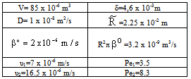
The catalytic membrane reactor in a flow-through mode also appears to be a promising process for industrial application[2]. A special case will be shown to demonstrate the role of the convective velocity in the membrane reactors. In this example, the membrane operates in dead-end mode and no separation procedure is performed. The task of the membrane is to provide for intensive contact between reactant and catalyst, combined with a short contact time and a narrow residence time distribution. Ilinitch et al.[11] have measured the reduction of aqueous nitrates using mono- and bimetallic palladium-copper catalysts impregnated in γ-Al₂O₃ support layers. The metal content was kept between 1.7 and around 7 w% with a particle size below 3-5 nm. The membrane layer is placed in a tank with stirring to circulate all feed solution through this membrane. The concentration of the reactant passing the membrane can be much lower than that in the feed phase. This value depends on the convective stream and the chemical reaction rate. The authors measured the nitrate conversion in three different modes, i.e. without convective flow and for two different values of convective flow with a surface velocity of 7 x 10^-6 and 16.5 x 10^-6 m/s (see Figure 12 in Ilinitch et al.[11]). For evaluation of the experimental results, the model A has been used with . It is easy to see that the outlet concentration is equal to the “bulk” concentration behind the membrane layer, as illustrated in Fig. 1b. The concentration change in the circulated reaction solution can be given as follows[C_L1 represents the bulk concentration denoted by in Eqs. (19) to (20)]:

(43)

The value of C_L1 denotes as the bulk concentration in the stirred tank. Its value changes as a function of time. The values of T and S parameters are given in Eqs. (19) and (20). Indicating the initial concentration of the reaction solution as C_Lo and solving Eq. (43), the following time function of concentration is obtained:

(44)

with

The data used for calculation are listed in Table 1.

Taking the diffusion stream through the membrane into account, the value of represents the residence time of the reaction solution as given by the following equation:

(45)

Performing the calculation using data from Table 1, the value of obtained was 400 min.

Table 1. Values of parameters used for calculation of the concentration change in the membrane layer[11,15]

Figure 10. Performance of catalytic membrane reactor situated in a perfectly mixed tank at different values of membrane Peclet number (points are measured data[11], lines are the predicted one)

The concentration of the reactant solution obtained was about 0.4 for the case of the diffusion driven mode (Pe=0) with Ф=1, whereas the value is around 0.08 for the case of the convective flow mode with Pe=10 at . These data are in line with the measured values, as can be seen in Fig. 10. The points represent the measured data whilst the continuous lines indicate the calculated values. It should be noted that the overall first-order kinetics was assumed for the nitrate-ion in the calculation. The H₂ concentration was kept constant during the reaction. The Ф values should be estimated for calculation of the conversion vs. time function. The value was obtained by fitting the measured conversion data from diffusion-driven flow (Pe=0). The continuous line for Pe=0 in Figure 10 was obtained using an estimated value of Ф=1.8. This value was then used for calculation of the curves for Pe=3.5 and 8. The continuous lines obtained by simulation are plotted together with the measured points. The calculated data for Pe=3.5 are slightly lower than the measured values, whereas the data obtained for Pe=8 are in surprisingly good agreement with the measured points. The good agreement between the measured and the calculated data proves that the model developed is suitable for estimating mass transport and conversion in the presence of both convective and diffusive flows.

4. Conclusions

A mathematical model has been developed in order to predict mass transport through a catalytic membrane reactor containing dispersed nanometer-sized catalyst particles using forced convective flow through the membrane layer, as well as for the case where the nanometer-sized catalytic particles are regularly dispersed in the membrane layer or the membrane intrinsically catalytic. Transport models developed include the mass transport into and inside the catalytic particles as well as through the catalytic membrane layer, taking into account both convective and diffusive flows. It has been shown that the two operating modes, namely with or without sweep phase on the permeate side can give essentially different inlet mass transfer rates. On the other hand, the application of the Fickian diffusive flow in the feed boundary condition in presence of convective flow can lead significant error in the mass transfer rate predicted. This error quickly increases with increasing boundary layer’s Peclet number due to the increasing curvature of the concentration distribution. Accordingly the application of the mass transfer coefficient predicted by the dimensionless number for the feed boundary layer should be avoided in the presence of forced convective flow. The models presented describe mass transport in good agreement with the measured data, proving that it can be used to estimate the mass transport process for a catalytic membrane reactor.

ACKNOWLEDGEMENTS

This work was supported by the National Development Agency grant (TÁMOP – 4.2.2/B-10/1-2010-0025)

Nomenclature

C = concentration in the membrane, mol/m³

C_i= concentration in the boundary layer, mol/m³ (i=1,2)

C_o= bulk concentration at t=0, mol/m³

= concentration on the catalyst interface, mol/m³

d_p= particle size, m

D= diffusion coefficient in the membrane matrix, m²/s

h= distance between particles, m

H = solubility coefficient of reactant between polymer matrix and the continuous phase,

H_d = solubility coefficient between catalytic particles and the membrane phase,

H_f = adsorption coefficient on the catalyst surface (=q/C), (mol/m²)/(mol/m³)

J_o = mass transfer rate without chemical reaction, mol/(m²s)

J = mass transfer rate into the catalytic membrane layer in presence of chemical reaction with constant diffusive flow in the boundary layers, mol/(m²s)

J_out = outlet mass transfer rate, mol/(m²s)

J_◊ = mass transfer rate obtained by variable diffusive flow, mol/(m²s)

j = mass transfer rate into catalytic particles, mol/(m²s)

k = reaction rate constant, 1/s

Pe = Peclet number or membrane Peclet number[Eq. (11)],

q = molar loading on the catalyst surface, mol/m²

R = particle radius, m

= radius of the membrane disc, m

V = volume of the reaction solution in the stirred tank, m³

y = space coordinate, m

Y = dimensionless space coordinate (=y/δ)

Greek letters

= physical mass transfer coefficient of the external phases, m/s (=D_i/δ_i with i=1,2)

= mass transfer coefficient of the polymer membrane layer (=D/δ), m/s

= physical mass transfer coefficient for diffusive plus convective flows,[Eq. (34)], m/s

= mass transfer coefficient for diffusive and convective flows,[Eqs. (23) and (39)], m/s

= mass transfer coefficient into particles defined in Eq. (10), m/s

= mass transfer coefficient of particles, m/s

δ = thickness of the membrane layer, m

δ_p = thickness of the diffusion boundary layer at the catalyst surface, m

ε = catalyst phase holdup

υ = convective velocity, m/s

Φ =reaction modulus (Eq. (11),

λ =dimensionless quantity after Eq. (14),

Θ =dimensionless quantity after Eq. (13),

Subscripts

f =interface

L =liquid

ov =overall mass transfer coefficient or rate

p = catalyst particle

1,2 =continuous phases on both sides of membrane

APPENDIX

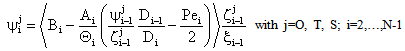
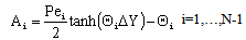
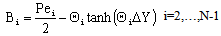
A second-order steady-state differential equation with variable (concentration dependent and/or local coordinate dependent) parameters and or in the case of nonlinear chemical reaction kinetics, e.g. Michaelis-Menten kinetics[Eq. (5)], can not be generally solved analytically. A numerical method or analytical approach can be recommended for its solution. Herewith we show a rather simple analytical approach where the mass transfer rate or the concentration distribution on side the catalytic membrane can be expressed in closed, explicit mathematical forms. For the solution the membrane layer should be divided into N sub-layers with constant parameters. This is illustrated in Fig. A1.

Figure A1. Important notations for the catalytic membrane divided into N sub-layer for linearization of e.g. Michaelis-Menten kinetics

The linearized form of the Michaelis-Menten kinetics can be as[13,14]:

(A1)

(A2)

The solution of this equation, according to Eq. (14), will be for the i^th sub-layer as (i=1,…,N):

(A3)

with

; ;

; ;

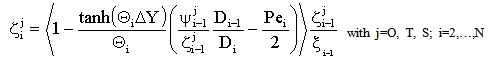
The T_i and S_i parameters can be determined by suitable boundary conditions. Neglecting the external mass transfer resistances, the boundary conditions can be given as[14]:

(A4)

(A5)

(A6)

(A7)

with

(A8)

The value of T₁ and S₁ for determination of the mass transfer rate

(A9)

(A10)

(A11)

(A12)

(A13)

(A14)

The initial values of and , namely and (j=T, S, O) are as:

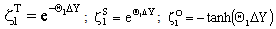(A15)

(A16)

The concentration distribution and/or the outlet mass transfer rate can also be easily determined. Applying the boundary conditions the other T_i and S_i values (i=2,…,N) can be determined[14]. Some calculations for the Michaelis-Menten kinetics are presented in Nagy’s book[14].