-
Paper Information
- Paper Submission
-
Journal Information
- About This Journal
- Editorial Board
- Current Issue
- Archive
- Author Guidelines
- Contact Us
American Journal of Chemistry
p-ISSN: 2165-8749 e-ISSN: 2165-8781
2025; 15(3): 64-75
doi:10.5923/j.chemistry.20251503.02
Received: Jul. 10, 2025; Accepted: Aug. 3, 2025; Published: Aug. 7, 2025

Modeling the Anti-Prostatic Activity of a Series of Turmeric Derivatives Using the Quantitative Structure-Activity Relationship
 Abstract
 Reference
 Full-Text PDF
 Full-text HTML
Pétah Ismaëli Aziz Do-Koné1, Nobel Kouakou N’guessan2, Georges Stéphane Dembele1, Kafoumba Bamba1, Abdoulaye Konaté2, Doh Soro1
1Laboratoire de Thermodynamique et de Physico-chimie du Milieu, UFR SFA, Université Nangui Abrogoua 02 BP 801 Abidjan 02, Côte-d’Ivoire
2Laboratoire Chimie Organique Structurale, UFR SSMT, Université Félix Houphouët Boigny BP 582 Abidjan 22, Côte-d’Ivoire
Correspondence to: Georges Stéphane Dembele, Laboratoire de Thermodynamique et de Physico-chimie du Milieu, UFR SFA, Université Nangui Abrogoua 02 BP 801 Abidjan 02, Côte-d’Ivoire.
| Email: |  |
Copyright © 2025 The Author(s). Published by Scientific & Academic Publishing.
This work is licensed under the Creative Commons Attribution International License (CC BY).
http://creativecommons.org/licenses/by/4.0/

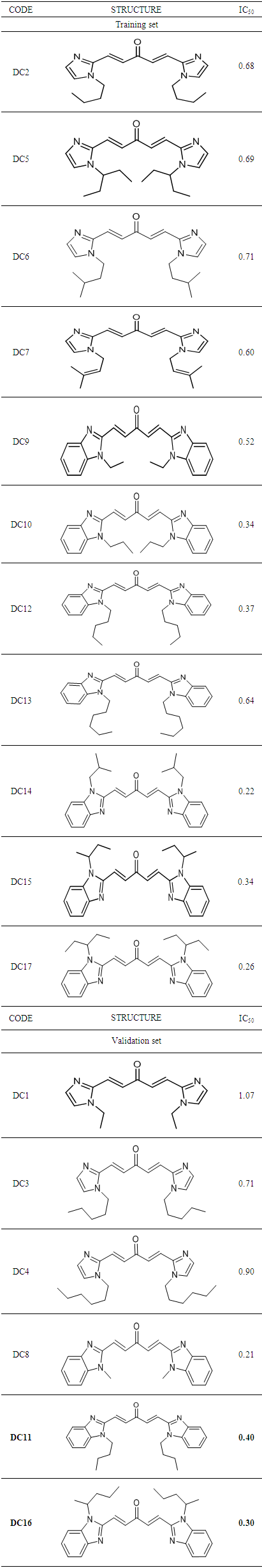
Curcumin derivatives are promising cytotoxic agents in the treatment of prostate cancer. The primary goal of this study is to establish a quantitative correlation between the structural features and anti-prostate activity of a series of sixteen (16) curcumin derivatives. Density functional theory (DFT) calculations at the B3LYP/6-31+G(d,p) level of theory were performed to determine the relevant molecular descriptors. The RQSA model developed using the multiple linear regression method (RLM) is a function of hardness (η), bond angle α(C-C=C), surface tension (TSurface) and density. Hardness (η) proved to be the most important descriptor for predicting the cytotoxic potential of the compounds studied. The statistical indicators associated with the model (R2=0.922; S= 0.068; F= 17.027) show that this model is robust with good predictive power. Our model's quality and performance were confirmed through internal validation using both leave-one-out (LOO) cross-validation and Tropsha criteria. This model is not due to chance and could be used to determine the cytotoxic activity of turmeric derivatives belonging to the same field of applicability.
Keywords: QSAR, Curcumin, Cancer, Prostate, DFT
Cite this paper: Pétah Ismaëli Aziz Do-Koné, Nobel Kouakou N’guessan, Georges Stéphane Dembele, Kafoumba Bamba, Abdoulaye Konaté, Doh Soro, Modeling the Anti-Prostatic Activity of a Series of Turmeric Derivatives Using the Quantitative Structure-Activity Relationship, American Journal of Chemistry, Vol. 15 No. 3, 2025, pp. 64-75. doi: 10.5923/j.chemistry.20251503.02.
Article Outline
1. Introduction
- Cancer encompasses a diverse group of diseases that can develop in virtually any organ or tissue of the body. Cancer develops through a multi-step process that transforms normal cells into malignant tumor cells, often progressing from precancerous lesions. Long considered “a disease of the rich”, cancer remains one of the world's most significant causes of mortality. According to the latest estimates from the International Agency for Research on Cancer (IARC), approximately 20 million new cases of cancer were detected internationally in 2022, and 9.7 million individuals succumbed to the disease [1]. The IARC also estimates that by 2050, the incidence of cancer worldwide is set to rise by 77%. The most common cancers in men are lung, prostate, colorectal, stomach, and liver cancers, while breast, colorectal, lung, cervical, and thyroid cancers are most common in women [1]. In our present study, we are interested in prostate cancer. The prostate is a gland of the male reproductive system whose volume increases with age. It lies below the bladder and in front of the rectum. It surrounds the beginning of the urethra, the channel through which urine and semen are evacuated. The prostate plays an important role in sperm production, producing a liquid called Spermatic fluid. The seminal vesicles, a pair of glands situated behind the bladder and above the prostate, are primarily responsible for producing the majority of the fluid that comprises semen. When initially normal prostate cells change and multiply in an uncontrolled way, forming a mass called a malignant tumor, this is called prostate cancer. At first, the mass is limited to the prostate. As the tumor progresses, it may grow larger and extend outside the prostate envelope. Cancer cells may break away from the cancer and travel via plasma or lymph spread to other parts of the body through blood vessels. This disease often progresses slowly, over several years. Prostate cancer develops without causing any particular symptoms. When the cancer is at an advanced stage, it may cause symptoms that raise suspicions of its presence, such as urinary tract infection, blood in the urine, urine retention, lower back pain or bone pain. For prostate cancer, family history has been identified as a risk factor. It has also been identified that men of Afro-Caribbean origin have an increased risk of developing this cancer. Occupational exposure to pesticides used in agriculture has also is known to contribute to the development of prostate cancer since the end of 2021 [2]. In Côte d'Ivoire, according to the national cancer control program (PNLCa), prostate cancer is the most common cancer among men, with nearly 2,757 new cases diagnosed, representing an incidence rate of 48.0 per 100,000 men in 2020 [3]. This mortality rate will continue to rise, as the latency of its symptomatology makes it a cancer that is often discovered late, and the clinical signs unfortunately reflect an advanced stage of the disease. To treat this cancer, several therapeutic methods are applied to patients, including surgery, radiotherapy, chemotherapy, targeted therapies, hormone therapy and immunotherapy. Castration and chemotherapy are the most frequently used because of the late stage of diagnosis. Treatment is tailored to each patient and depends on the tumor's potential to progress. Localized tumors can be treated curatively by surgery (total prostatectomy) or radiotherapy (external or brachytherapy). Locally advanced tumors are treated with a combination of radiotherapy and hormone therapy. Metastatic tumors can be treated with hormonal therapy. Chemotherapy and, increasingly, second-generation anti-androgens are used to treat castration-resistant forms. Chemotherapy remains the best alternative due to the more or less effective anti-cancer drug treatments based on docetaxel, mitoxantrone and cabazitaxel [4]. However, these molecules come up against resistant strains of prostate cancer. Hence the urgent need to find other anti-cancer agents with improved properties. The plant kingdom abounds in a number of natural compounds with efficient biological and medical properties. Curcumin is a phenolic compound identified in the rhizome of turmeric. Turmeric is a rhizomatous herbaceous plant that rhizomes have been used for many years in cultural Indian remedy and Asian cooking. Turmeric is part of the Asian diet, and it has been discovered that Asians have developed resistance to prostate cancer thanks to their consumption of turmeric [5]. As a result, scientists were able to identify curcumin as the main molecule responsible for turmeric's anti-prostate cancer activity [6]. Having shown a capacity to prevent prostate cancer, in 2000 curcumin was tested on cell culture systems in vivo and in vitro as a potential treatment for prostate cancer [7]. Like many other researchers, Rubing Wang et al. in 2015 investigated the anti-prostate cancer activity of curcumin derivatives. Their study, which focused on a series of curcumin analogs derived from (1E,4E)-1,5-di(1H-imidazol-2-yl)penta-1,4-dien-3-one, showed that these compounds effectively led to apoptosis of hormone-refractory metastatic PC-3 prostate cancer cells [8]. Therefore, in order to anticipate any resistance by designing curcumin derivatives with improved anti-prostatic activity, it is important to identify the origin of the anti-cancer properties of curcumin derivatives. This is the context of our study, the general aim of which is to model the anti-prostatic activity of a series of curcumin derivatives. The aim is specifically to found a quantitative structure activity relationship (QSAR) to explain the cytotoxicity of a series of sixteen curcumin derivatives whose anti-prostatic activities have been determined experimentally (Table 1) [8]. The QSAR methodology used in this work is a valuable tool for predicting and understanding the cytotoxicity of compounds for pharmaceutical interest.
|
2. Materials and Experimental Procedures
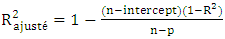
- Data collection methodsModeling the anti-prostatic activity of curcumin derivatives requires the determination of descriptors. An infinite number of descriptors exist, including 2D and 3D descriptors. The 2D descriptors used in our model are derived from the compounds' 2D structure obtained with ChemSketch [9]. The 3D descriptors are determined from the optimized structure of the compounds. Optimization and frequency calculation are performed using Gaussian 09 software [10]. For these various calculation operations, density functional theory (DFT) is used at the B3LYP/6-31+G(d,p) level [10]. This level conceptual is a combination of the hybrid three-parameter Lee-Yang-Parr functional and the double split valence basis with polarization effects on heteroatoms. In addition, the multilinear regression method implemented in XLSTAT software version 2014 [11] was used to develop the QSAR model.Molecular descriptorsVarious physico-chemical descriptors can be used to develop QSAR models. However, in our study, we used a descriptor derived from the global reactivity of compounds and 3D and 2D geometric descriptors. Chemical hardness is a valuable tool for understanding and predicting the behavior of molecules in various chemical environments. It measures a molecule's resistance to electronic deformation during chemical reactions, expressing in other words a system's resistance to changes in its electron number. It is therefore a measure of a molecule's stability against nucleophilic and electrophilic attack. A hard molecule is less reactive, while a soft molecule is more reactive. Its expression is as follows:
 | (1) |
 and the density of the molecule. The descriptor bond angle α(C-C=C) is illustrated in the figure. Surface tension is a fundamental property of liquids that influences many physical and chemical phenomena. Surface tension is fundamental to biochemical reactions such as respiration (gas exchange in pulmonary alveoli) or substance transport in blood vessels. Density is a fundamental property that helps us understand the characteristics of molecules and their behavior in various media.
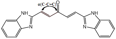 | Figure 1. Geometric descriptor for curcumin analogues |
 | (2) |
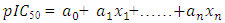
 (i =1,…, n) are the coefficients of the regression parameters and
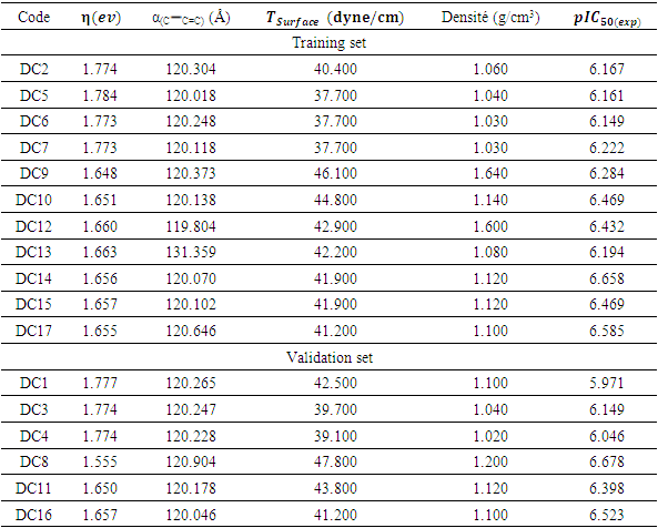
  is the constant of the model equation.The multiple linear regression method proved useful for expressing the IC50 inhibitory activity of DC as a function of descriptors. It is essential that the descriptors are independent of each other to guarantee the efficiency of the model. To achieve this, the partial correlation coefficient
  between the values of descriptors i and j should be less than 0.70
  [13]. It is determined according to the following relation.
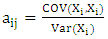 | (3) |
 | (4) |
 | (5) |
 | (6) |
 | (7) |
 | (8) |
 | (9) |
 | (10) |
 [17]It quantifies the predictive power of the model on training data.
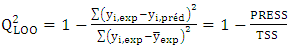 | (11) |
 [17]This criterion evaluates the model's ability to make accurate predictions on the test set.
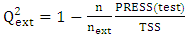 | (12) |
 | (13) |
 | (14) |
 | (15) |
 [20]By evaluating this parameter, we can tell whether the pattern is the product of chance or not. A value is larger than 0.5indicates that the model is significant and not by chance.
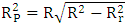 | (16) |
 the mean value of the
  of the models generated using random parameters. For the prediction to be acceptable, the value of the metric
  must be less than 0.20 when that of
  is greater than 0.50.
 | (17) |
 | (18) |
 | (19) |
 and
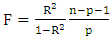
and  represent the coefficients of determination Between observed and predicted values, with and without interception respectively. In addition to internal validation, external validation is also required. It is carried out by using the ratio (theoretical activity) / (experimental activity) and the Tropsha criteria.Ø Tropsha criteria [20] [21]There are five Tropsha criteria:
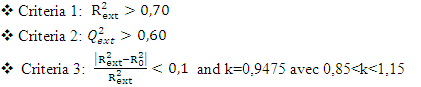 | (20) |
 | (21) |
 | (22) |
 Coefficient of determination for the molecules in the test series;
 Coefficient of determination of the regression model for the test set;
 Coefficient of determination of the regression among experimental and predicted values for the test series; k: Slope of the correlation line (predicted values vs experimental values); k': Slope of correlation line (experimental values vs. predicted values).QSAR model applicability domain:The applicability domain of a QSAR model is established using the threshold lever [22]. The concept of leverage is essential for assessing the validity and robustness of QSAR models, helping to identify data points that could disproportionately influence model results. Leverage” refers to a parameter that measures how much a specific data point influences model predictions. A point with high leverage has a disproportionate impact on model results. Leverage is often calculated from the model's matrix of explanatory variables. It is related to the interval of a point from the mean of the points in the variable space. For observation i, it should be calculated as follows:
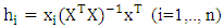 | (23) |
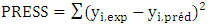
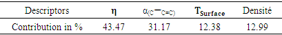
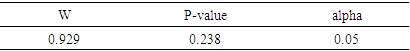
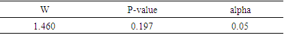
 [23], where N signifies the sample size of the training set, and k indicates the number of independent variables used in the model. A compound is considered outside the model's applicability domain if its residual and leverage exceed the critical h* value. Normality testNormality tests are statistical techniques used to evaluate the hypothesis that a given sample originates from a normally distributed population. A wide range of parametric statistical tests, such as t-tests and ANOVA, are based on the normality assumption, which stipulates that the data are normally distributed. Testing this assumption is essential to guarantee the validity of the results. Normality testing helps to understand the probability distribution of the data, and assists to select the appropriate statistical methods for analysis. Normality tests are essential for validating statistical analysis hypotheses. If the data fails to meet the normality assumption, non-parametric statistical tests, which do not rely on the assumption of a normal distribution, can be employed. In practice, for example, verification of the normality of residuals in linear regression is rarely carried out, although it is essential to guarantee the reliability of confidence intervals for parameters and predictions. This normality of residuals can be verified by analyzing certain graphs, or by using a normality test that relies on the independence of residuals using certain graphs [24].Shapiro-wilk testThe Shapiro-Wilk test [25] is a statistical procedure used to test the hypothesis that a given sample originates from a normally distributed population. The test is based on two competing hypotheses: the null hypothesis, which assumes that the data follows a normal distribution, and the alternative hypothesis, which suggests that the data does not follow a normal distribution.• The null hypothesis(H0) posits that the data are drawn from a population that is normally distributed.• The alternative hypothesis (H1) posits that the data are not drawn from a population that is normally distributed.Generally recommended for small sample sizes (n < 50), but can be used up to n = 2000. The test uses the correlation coefficients between the observed data points and the theoretical values of a normal distribution. The result is a W statistic, which varies between 0 and 1. The p-value obtained is compared with a threshold, often set at 0.05:• p-value < 0.05: Rejection of the null hypothesis, data are not normally distributed.• p-value ≥ 0.05: No rejection of the null hypothesis, data can be considered as normally distributed. Application of this test to the predicted cytotoxic activity values of the established model produced the following results in XLSTAT software [11].Probability-probability graphA probability-probability plot (Q-Q plot, or quantile-quantile plot) is a graphical method used to compare the empirical distribution of a dataset to a theoretical distribution, such as the normal distribution. It is often used in conjunction with normality tests such as the Shapiro-Wilk test. The Q-Q plot is utilized to test for normality. The Q-Q plot visually compares the empirical quantiles of the dataset to the theoretical quantiles of a specified distribution. with those of a theoretical distribution. The Q-Q Plot is constructed in two stages: calculating quantiles and plotting points: On a graph, the quantiles of the observed data are placed on the y-axis and the quantiles of the theoretical distribution on the x-axis. If the points are collinear, they all fall along the same straight line (usually the diagonal), this indicates that he data follow a normal distribution pattern, characterized by a symmetric, bell-shaped curve centered around the mean.Contribution of an explanatory variable to the prediction of an activityThe contribution of the explanatory variable
  , denoted by
  to the prediction of activity Y [24] [25] is evaluated by Student's t test, allowing us to determine its relevance in the model. It measures the importance or contribution of variable
  in the QSPR/QSAR model according to the following relationship:
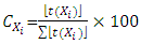 | (24) |
3. Resultats Et Discussion
- A series of sixteen curcumin derivatives are being investigated for their anti-prostatic activity. In order to carry out our QSAR study, this experimental database was split into two groups. The first group, comprising 11 molecules (i.e. 2/3 of the database), constitutes the training set. The second group, comprising 5 molecules (1/3 of the database), is called the validation set. The values of the descriptors and the cytotoxic activity of the molecules are given in Table 2.
|
|
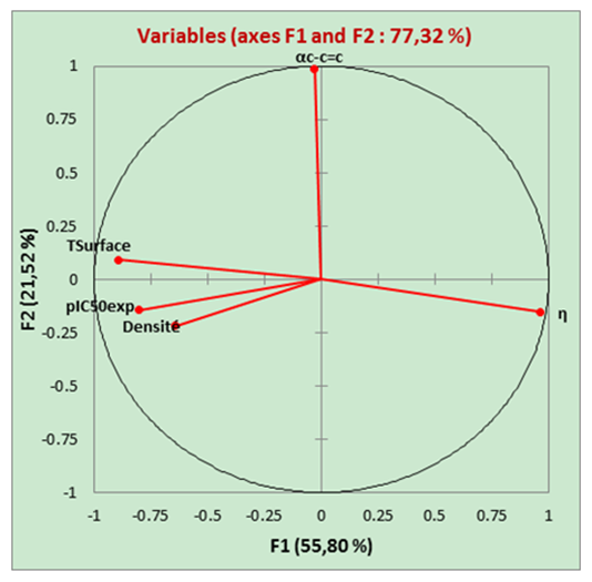 | Figure 2. Correlation circle |
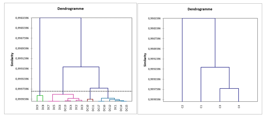 | Figure 3. DC dendrograms |
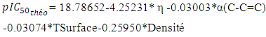 | (25) |
|
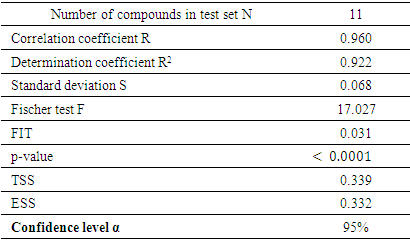
 depends on hardness, angle, surface tension and density. The model's regression equation shows negative coefficients for all variables namely η, α(C-C=C), TSurface and density. These negative coefficients indicate that cytotoxic potential increases as the values of these descriptors decrease. In other words, inhibitory concentration is enhanced for a smaller value of these descriptors. Analysis of the statistical parameters associated with the QSAR model indicates a correlation coefficient R of 0.960. This high value highlights a strong linear correlation between inhibitory activity and the descriptors used in the model. Moreover, 92.22% of the experimental variable
  this is elucidated by the the model incorporates various descriptors (R2 = 0.922). Furthermore, a standard deviation (S= 0.068) tending towards 0 indicates a good fit and high predictive reliability. The high Fischer test value (F = 17.027) is well above the critical value derived from the Fischer table, confirming the significance of the model. Also, parameter values such as the experimental variance (TSS = 0.339) and the variance due to the model ESS = 0.332 indicate that there is less variability in the data.
|
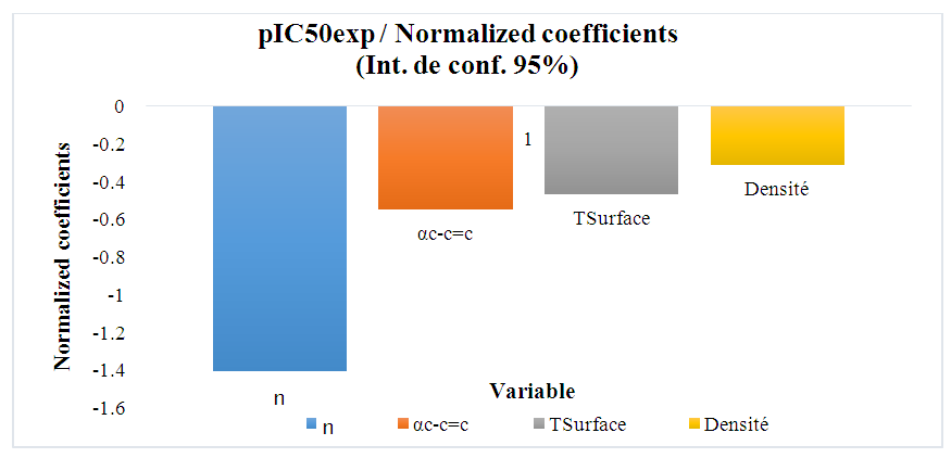 | Figure 4. Standardized descriptor coefficients |
|
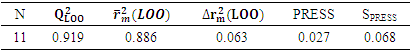
 , which is greater than 0.50, indicates that 91.90% the molecules in the test set exhibit their cytotoxic potential perfectly predicted by the model. The model displays a high predictive ability in relation to the molecules included in the training set for model training. Consequently, this result indicates that the model exhibits low sensitivity to the operation of isolating a molecule before reintegrating it into the learning set (Leave-One-Out). The value of
  is greater than 0.50 while that of
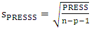
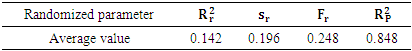
  is less than 0.2. Thus, the model is considered sufficient for use in predicting cytotoxic potential. The low value of the SPRESS error indicates a good model.• Y-randomization testTo ensure that the model is not random, we carried out a randomization test, which consisted in performing a circular permutation in the training set. The table 7 displays the values of the randomization parameters following 10 iterations.
|

 is low (
 =0.142), Showing that the equation for the regression line explains only 14.20% of the distribution of points (cytotoxic potential). The high standard deviation (sr=0.196) also points to a dispersion of points around the regression line.
  The value of Roy's parameter
  , 0.848 (exceeding 0.50), confirms that the model's performance is statistically significant and not attributable to random variation.
|
|
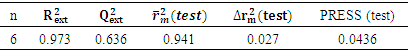
 which is 0.636 indicates a prediction rate of cytotoxic potential of 63.60%. In order to
  , It holds a value higher than 0.50 while that of the other is
  is less than 0.2 we can therefore conclude that the model is acceptable to estimate the future value of the cytotoxic the capability of the molecules in the validation set. To further assess the robustness of our model, the five (05) Tropsha criteria are calculated.• Checking Tropsha criteriaCriteria 1:
 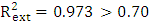 Criteria 2:
 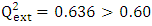 Criteria 3:
  Criteria 4:
  Criteria 5:
 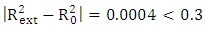 It is clear that all five (05) Tropsha criteria are met. Consequently, the model developed is extremely effective in predicting the potential for the initial reduction.Correlation between model-predicted values and experimental valuesTheoretically calculated pIC50 values and experimentally determined pIC50 values are compared using the correlation curve (figure 5).
|
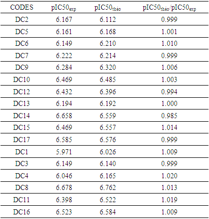
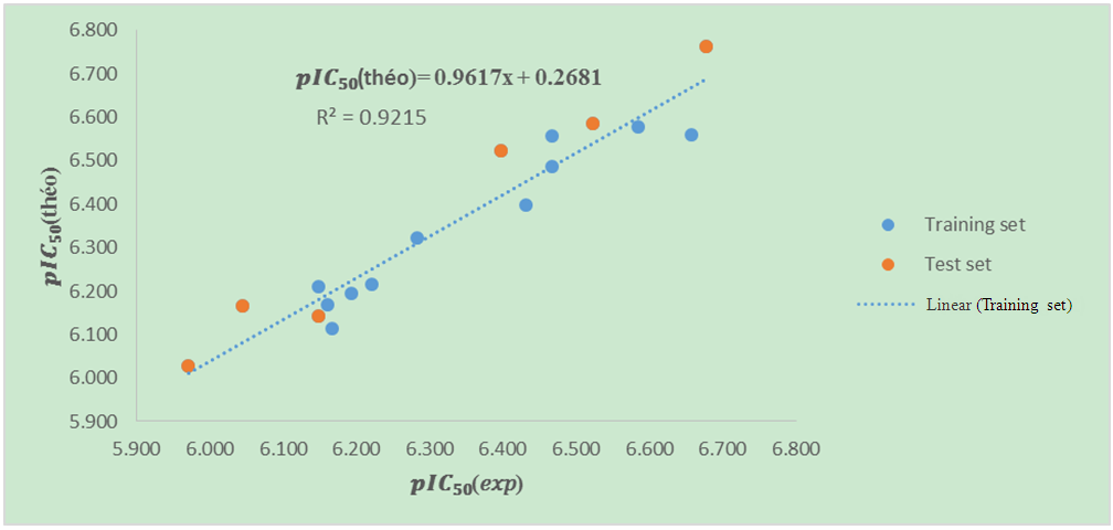 | Figure 5. Correlation curve between 𝒑𝑰𝑪𝟓(𝑒𝑥𝑝)-𝒑𝑰𝑪𝟓𝟎(theo) model |
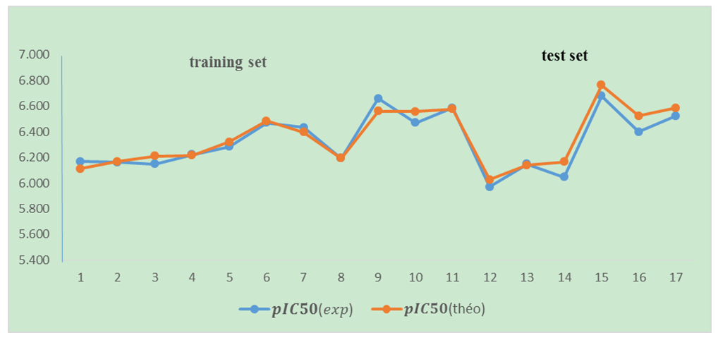 | Figure 6. The match between the model-predicted values and the experimental results |
|
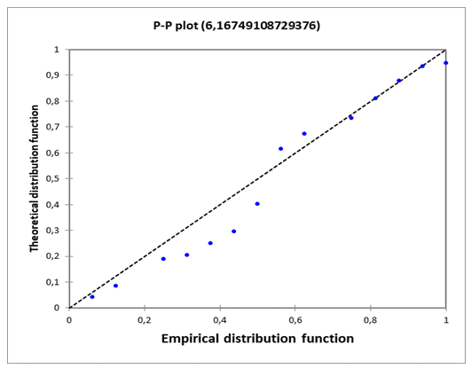 | Figure 7. P-P plot (𝒑𝑰𝑪𝟓(theo)) of the mode |
|
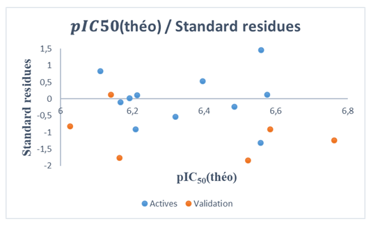 | Figure 8. Normalized residuals graph=f(𝒑𝑰𝑪𝟓𝟎 (theo)) of the model |
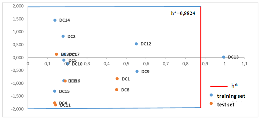 | Figure 9. Williams diagram of the model |
 . Although this last observation presents an atypical value, it does not necessarily constitute an anomaly for the model. Influential observations, such as those identified by high leverage, can improve model accuracy provided their impact on residuals is limited. The results obtained with the RQSA model indicate a good fit to the data, with no evidence of outliers likely to bias the analyses. Cross-validation and applicability domain analysis demonstrate that the model is robust and can be used to make reliable predictions on new DC molecules.
4. Conclusions
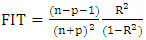
- Curcumin is a compound of interest in the development of cytotoxic agents effective against prostate cancer. The aim of this work was to rationalize the anti-prostate activity of curcumin derivatives with a view to improving it. A quantitative structure-activity relationship was established for a series of sixteen curcumin derivatives. The model developed using the multilinear regression method is a function of hardness η, angle α(C-C=C), surface tension TSurface and density, which help to explain the property. In addition, anti-prostate activity is intimately related to hardness and angle α(C-C=C). The model is accredited with good static indicators (R = 0.960; R2 = 0.922; F = 17.027; FIT = 0.031) highlighting excellent predictive power. Also, internal and external validation of the model elucidated its robustness and predictive power. This model is not due to chance, and follows a normal distribution law. Thus, as part of the process of designing cytotoxic agents with improved activity, this elaborate model is suitable forecasting the activity of curcumin derivatives not yet synthesized or whose activity has not yet been determined. As a follow-up to this work, we plan to carry out molecular docking to explain the activity of these compounds in interaction with the protein responsible for prostate cancer.