1. Introduction

Correct data management and/or pre-processing as well as rigorous statistical analysis represent a crucial steps for a right statistical data analysis in experimental sciences. Nowadays, whole sequencing survey based on next generation sequencing (NGS) approaches allowed the development of strong bioinformatics and bio-statistical (computational bio-statistic) tools with the purpose to appropriately manage impressive amount of qualitative and as well quantitative data by saving time [1]. Indeed, bioinformatics and computational biostatistics research fields result to be in expansion, because of the impressive number with regard genomic and transcriptomic research projects [1, 2]. Thus, it is basically inconceivable to dissolve biology with computational statistics. Statistical analysis with regard experimental biology results is often qualified as a constraint and as well a necessary but unpleasant passage. However, the first objective of the statistics in biological survey is to reveal what the data must tell us. Also, with advances in life sciences as well as in agronomic disciplines and/or sciences, it has become commonplace to generate large multidimensional datasets requiring strong, quick and rigorous statistical analysis scheme [3]. In addition, the impressive amount of collected data during biological experimentations as well as that data heterogeneities could complicate the underlying statistical analyzes. So, this typology of analysis needs a rigorous scheme with regards data pre-treatment and/or pre-processing and as well organization. Hence, data management in biological experimentations remains a delicate phase, since it could condition decision taking in statistical hypothesis test. Considering as a whole, data heterogeneity issues, make statistical analysis more complex in biological and as well agronomic experimentations and request an accurate computational statistical scheme and as well methodology with the purpose to optimize and improve statistical analysis results. Usually, the first step in statistical survey is to gather and organize raw data. R programing environment offers a graphical interface that allows diverse datasets to be directly captured [4]. Nevertheless, advances in informatics technology and as well impressive data amount in biological experimentations have propelled the integration between both informatics and statistic sciences. Several authors provided computational statistical tools for morphometric data processing and/or management [3, 5, and 6]. Measuring shape and size variation is essential in life science and in many other disciplines. Since the morphometric revolution of the 90s, an increasing number of publications in applied and theoretical morphometric emerged in the new discipline of statistical shape analysis [4]. The R language and environment offers a single platform to perform a multitude of analyses from the acquisition of data to the production of static and interactive graphs [7]. This offers an ideal environment to analyze data variation through a simple and explicit graphic representation. This open-source language is accessible for novices and for experienced users. Adopting R gives the user and developer several advantages for performing morphometric adaptability, interactivity, a single and comprehensive platform, possibility of interfacing with other languages and software, custom analyses, and graphs. There are many text books web pages that can be used to learn basics of the R environment, such as (i) Getting started with R’ [8], (ii) quite comprehensive The R book [9] or (iii) Quick-R webpage (http://www.statmethods.net/) and manuals on R homepage (http://cran.r-project.org/manuals.html) [7]. We have thus developed a statistical analysis pipeline in order to bring together in the same environment a series of R software functions allowing to a category of biologists (especially those of our research team with weak programming skill) who are new to programming as well as without any programming skill, to have at their disposal a powerful and simple and comprehensive multivariate statistical analysis scheme and tool, guaranteeing correct statistical result and/or data interpretation. In this analysis, the pipeline has been tested by processing our old data set (Appendix file 1), which results have been published by Diarrassouba et al. (2015) and Dago et al. (2016), providing readers and/or users to check the latter accuracy. Presently developed computational statistical pipeline by including several R libraries, is executed in three great steps: (i) experimental raw data loading (input data), (ii) automate data processing and statistical analysis and (iii) results (output files) as summarized in appendix file 2. Even if the present pipeline processed an agronomic quantitative data set (appendix file 1) it is noteworthy to underline it usefulness and as well applicability for any generic quantitative data set.

2. Materials and Methods

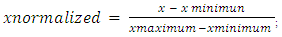
Preamble

The pipeline has been developed in R version 3.3.1 (2016-06-21) with the following reference; "Bug in Your Hair" Copyright (C) 2016 the R Foundation for Statistical Computing Platform: x86_64-w64-mingw32/x64 (64-bit). The first step of any statistical and as well metric data analysis is to gather and organize raw data. User can prepare and/or organize manually data matrix to be submit to the pipeline, contributing to less computational attitude of the latter (developed pipeline). In the other words, user can interact with the pipeline workflow. However, R programming language offers a graphical interface that allows diverse datasets to be directly captured from work directory named; dir. So, dir () function recalls objects recorded the work environment and/or in the directory. Processed data may gather in an appropriate way before assigning them to R objects. The quality of data acquisition determines part of the quality of the results: measurement error results both from the user and from the accuracy of the different tools used for measuring data. It may happen that data are incomplete for some objects. Data pre-treatment step is needed by the user before loading row data matrix file for descriptive as well as clustering and analytical statistical analysis. Also, data matrix file to be uploaded must be converted in test file and saved with .csv and/or .txt extension (for this analysis row data matrix has been converted in text file with .txt extension). However, coma “,” character indicating decimal number in row data matrix, must to be converted in dot, if any, by using gsub R function as following: gsub(“,”, “.”,matrix.data)-> New_matrix; where “matrix.data” represents numeric matrix containing row data including decimal number with “,” character. Also, dec="," function in reading data matrix easily solve above mentioned concern (see below in result and discussion chapter).

Installation

R and additional packages can be downloaded from http://www.r-project.org/. Follow the instructions on the R web page. All functions described here were tested with R version 3.3.1. In working with R, it is possible to directly use the console version you will install. However, other software can communicate with R and handle your data in more conveniently. We recommend R Studio (http://www.rstudio.com/), which, among other features, allows for the easy editing of R scripts and the running of selected parts of the script, highlights the syntax, and provides an instant list of objects and functions in the current environment.

Apart from the base R installation, download and install the following additional packages: ade4, class, permut, scatterplot3d, and vegan. The packages are most easily downloaded and installed from the menu Packages Install packages.

External packages installation

Some of the features presented in the pipeline require you to install packages that are not supplied with the basic R distribution such as Gplots [10], Ape [11], Psych [12], Factor Min R [13] and R Color Brewer [14] and as pvclust an R package for hierarchical clustering with p-values [15].

Package installation

Internet connection is required to install packages, since it must be downloaded from a server. Package installation is done only once. So by using R console, install.packages allows to choose a sever connection ("package") for package downloading. Austria is the one that is updated most quickly. However, the other packages record an acceptable update frequency. Also, using R console needed packages installation procedure requires two steps as following: (i) download the package sources from its repository, the main site being the CRAN (Comprehensive R Archive Network): http://cran.r-project.org in the packages section; (ii) install the package by typing R CMD INSTALL package where the term package is for the name of the tar.gz file containing the sources. It is noteworthy to underline that procedure explained here is the simplest. For more information with regard other R package installation procedure reader and/or user can see the FAQ and/or http://cran.r-project.org/doc/manuals/R-admin.html#Installing-packages link.

Loading of the package

R package loading is needed for each session where it must be used. The command with regard package loading procedure is simple and is as following; library (package); where the term package is referred to processed package name.

Update installed packages

Automatic updating procedure with regard all installed packages can execute by running update. packages (ask = FALSE) script. After that, R will downloads all the updates. Also, regular update of R platform packets is necessary for a better exploitation of the latter’s.

Data treatment support

R is multiplatform running in Windows (from XP), Linux and Mac systems. At the processor level, R software is compatible with 32-bit and 64-bit processors. Data treatment procedure via presently developed pipeline require a calculator with a RAM capacity around 256 MB at least. However it is recommended to have RAM capacity higher than 1GB for the use of the pipeline allowing to process large amounts of data. The present pipeline have been implemented in Windows (from XP) system.

Pipeline methodology

(i) Data preparation

It is important to define clearly processed experimental data condition. In the other words, experimental variables that will be taken into account by the pipeline for statistical analysis must be well specified (first line of table containing row data). Statistical methodologies used in this work concern quantitative agronomic metric data from our previous investigations [16, 17] (see appendix 1).

(ii) Experimental design

Experimental design is needed for experimentation studies. The experimental design includes factors and/or parameters that influence the experimental conditions, the number of repetitions to be performed and as well the experimental design scheme. Also, class combination with regard several factors in an experimental design constitutes a treatment.

(iii) Row data matrix

A correct data structuration as well as data collection contribute in avoiding to introduce a bias in statistical analysis. Then, correctly structured data matrix is an important step in the research study. In this scheme it is mandatory to clearly identify quantitative variables and factors, as well as that factors classes. Once this discrimination is done, it will result in an easy statistical analysis. In general, it is prudent to build data table matrix in a spreadsheet allowing dataset management in an external source with regard R software (Appendix 1). Also, in the spreadsheet, individual features must be placed in rows and variables in columns.

(iv) Data loading

Let us assume that the data file(s) are named genotypes.txt and coordinates.txt and stored in a directory called data. Then type in the R environment: geno<- read.table (".../data/genotypes.txt", na.string="000") ## change "000" to according to your file... the genotypes are loaded and stored in an R object called geno. Then type again in the R environment: coord <- read.table (".../data/coordinates.txt") ... the coordinates are loaded and stored in an R object called coord. Generally you can replace .../data by any string path to my data giving the path to the data relatively to the working directory. Under Windows this working directory is specified through the manual and sub-menu preferences. Under Linux, the R working directory is the Linux working directory of the terminal from which R was launched.

Statistical functions of the Pipeline

Heterogenic agronomic metric data normalization

In statistics and applications of statistics, normalization can have a range of meanings [18]. In the simplest cases, normalization of ratings means adjusting values measured on different scales to a notionally common scale, often prior to averaging. In more complicated cases, normalization may refer to more sophisticated adjustments where the intention is to bring the entire probability distributions of adjusted values into alignment [6, 18]. There are several types of standardization. Users are free in using data standardization method fitting better for their analysis (data). Here, we used normalization system (random chosen) that consists in centering and reducing the data of each variable column in the interval [0-1]. In this system, the minimum value of a data series is 0 and the maximum value 1. Mathematical formula with regard above mentioned normalization system is as following:

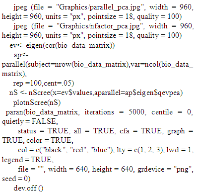
Assessment of processed data clustering and distribution by multivariate boxplot and hierarchical clustering analysis

Boxplot graph allows to assess processed data dispersion by identifying outliers data and/or sample (data quality control). The boxplot function allows to build boxplots in base R. Boxplot is one of the most common type of graphic. It gives summary of one or several numeric variable. Indeed, the line that shares the box into 2 parts represents the median of process data while both upper and lower bases of the box shows the upper and lower quartiles respectively. The extreme lines shows the highest and lowest value excluding outliers.

Hierarchical cluster analysis, is an algorithm that groups similar samples into groups called cluster. Hierarchical clustering can has been performed on raw and normalized genetic features data. Once data are provided, the pipeline automatically compute a distance matrix in the background. Usually, distance between two clusters has been computed based on length of the straight line drawn from one cluster to another. This is commonly referred to as the Euclidean distance. Here, the hierarchical survey based on the Euclidean distance, as it is usually the appropriate measure of distance in the physical world.

Correlation tests

In the present pipeline several correlation coefficient have been evoked depending on processed data typology. Correlation coefficients are used in statistics to measure how strong a relationship is between two or more variables. There are several types of correlation coefficient: Pearson’s correlation is a correlation coefficient commonly used in linear regression. The value of correlation is numerically shown by a coefficient of correlation, most often by Pearson’s or Spearman’s coefficient, while the significance of the coefficient is expressed by p-value. The coefficient of correlation shows the extent to which changes in the value of one variable are correlated to changes in the value of the other. Spearman's coefficient of correlation or rank correlation is calculated when one of the data sets is on ordinal scale, or when data distribution significantly deviates from normal distribution and data are available that considerably diverge from most of those measured (outliers) [5, 19, 20]. Spearman rank correlation is a non-parametric test that is used to measure the degree of association between two variables. The Spearman rank correlation test does not carry any assumptions about the distribution of the data and is the appropriate correlation analysis when the variables are measured on a scale that is at least ordinal while Kendall rank correlation is a non-parametric test that measures the strength of dependence between two variables [21]. Also, it is noteworthy to underline that presently developed pipeline provides processed correlation heatmap as well as phylogenetic tree graphic.

Parallel Principal Component Analysis (PCA)

A first essential step in Factor Analysis is to determine the appropriate number of factors with Parallel Analysis. Parallel PCA survey and/or technique is realized with the purpose to evaluating the components or factors retained in a principle component analysis (PCA) or common factor analysis (FA). Evidence is presented that parallel analysis is one of the most accurate factor retention methods while also being one of the most underutilized in management and organizational research. Specifying too few factors results in the loss of important information by ignoring a factor or combining it with another [22]. This can result in measured variables that actually load on factors not included in the model, falsely loading on the factors that are included, and distorted loadings for measured variables that do load on included factors. Furthermore, these errors can obscure the true factor structure and result in complex solutions that are difficult to interpret [23, 24]. Several studies have shown that parallel analysis is an effective method for determining the number of factors. Despite being the most critical, top priority issue of factor analysis, determining the number of factors has been considered as one of the most challenging stages; this is particularly true for researchers inexperienced in factor analysis, although it is occasionally difficult for many experienced researchers, depending on the characteristics of the instrument (or scale), the research group and thus the collected data [25-29]. Essentially, the program works by creating a random dataset with the same numbers of observations and variables as the original data. A correlation matrix is computed from the randomly generated dataset and then eigenvalues of the correlation matrix are computed. When the eigenvalues from the random data are larger than the eigenvalues from the pca or factor analysis you known that the components or factors are mostly random noise.

3. Results and Discussion

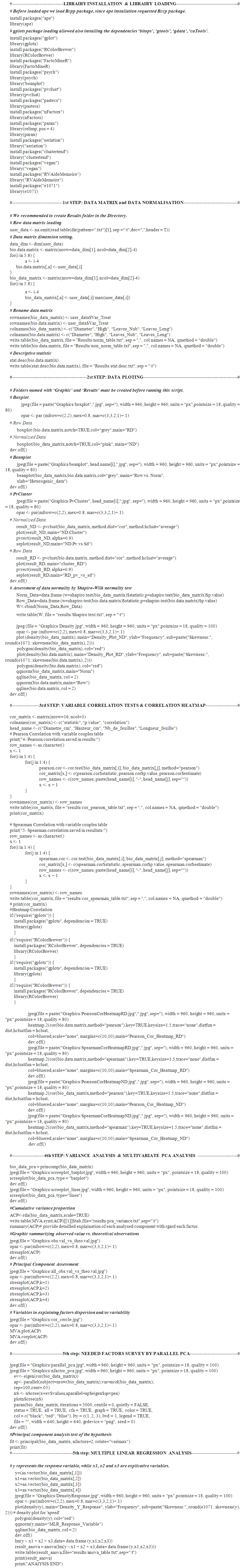
In prelude: we notify that “#” character in the pipeline introduce a comment line. Also, the pipeline requests and/or needs several libraries installation and loading before running (see below). Mean applications of presently developed pipeline will be considered as sub-chapters of results and discussion chapter.

3.1. Data Matrix Loading Process and First Data Analysis

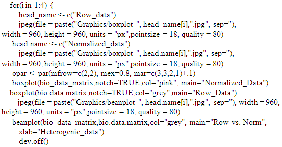
Once row data table and/or row data matrix has been adequately prepared (i.e. appendix file 1) (see also the material and methods chapter), data are loaded in R console and/or working area. Next, data are submitted to a standardization procedure with the purpose to overcome bias in subjacent statistical analysis because of that data heterogeneity (the present pipeline is flexible, allowing users to choose standardization systems fitting well to their data set). Boxplot and bean-plot graphics (multiple descriptive statistic) provided a visual comparative analysis between (i) standardized and unstandardized (row) data. The pipeline provide pvclust R package for assessing the uncertainty in hierarchical cluster analysis. Pvclust performs hierarchical cluster analysis via function it hclust function (see script on the pipeline) and automatically computes p-values for all clusters contained in the clustering of original data. This survey function provides graphical tools such as plot function or useful pvrect function which highlights clusters with relatively high and/or low p-values. So, pipeline functions involving in aforementioned analysis are reported as following:

# Memory clean up.

rm(list=ls())

# Start the stopwatch

ptm <- proc.time().

# Needed libraries loading

install.packages("ape")

Library (ape)

library (gplots)

library (RColorBrewer)

install.packages("FactoMineR")

library (FactoMineR)

library (psych)

library ('beanplot') # [30]

install.packages("pvclust")

library(pvclust)

install.packages("pastecs")

library(pastecs)

install.packages("paran")

library(relimp, pos = 4)

library(paran)

install.packages("nFactors")

library(nFactors)

install.packages("seriation")

library("seriation")

install.packages("clustertend")

library("clustertend")

install.packages("vegan")

library("vegan")

install.packages("RVAideMemoire")

library("RVAideMemoire")

nstall.packages("e1071")

library(e1071)

# Data matrix loading (here data matrix *.txt format).

Users should prepare adequately row data matrix with txt extension (see appendix file 1) in the work directory. Also, the users must to create two folders named (i) Results (tables saving area) and Graphics (graphic saving area) before running the pipeline. Users can change the nomenclatures of above mentioned folders, paying attention to adjust it in the whole pipeline, this due to pipeline flexibility. As the script below, “user_data” represents the new name of matrix containing row data by processing and/or running the pipeline.

user_data <- na.omit(read.table(dir(pattern=".txt")[1], sep ="\t", dec=",", header = T))

# Data matrix size retrieving.

Here, we used integer number in referring to data matrix column (see appendix file 1).

# “dim” allowed to retrieve row data matrix dimension.

data_dim <- dim (user_data)

data_matrix <- matrix (nrow=data_dim[1], ncol=(data_dim[2] - 4)) # New matrix dimension.

# New performed matrix will include data_dim[1]= 96 row and data_dim[2] – 4= 4 column (appendix 1).

# News data matrix including row data.

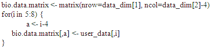# New data matrix including maximum normalized data.

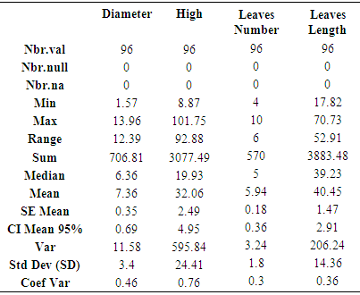
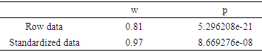
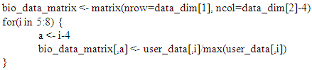# Matrix parameters and variables name assignment.

Here the pipeline give an opportunity to users to adapt and/or adjust and as well to change analyzed variables names.

rownames(bio_data_matrix) <- user_data$Var_Treat # Var_Treat row from loaded “user_data” matrix have been processed as the new matrix (matrix with row data) row names.

rownames(bio.data.matrix) <- user_data$Var_Treat # Var_Treat row from loaded “user_data” matrix have been processed as the new matrix (matrix with normalized data) row names.

colnames(bio_data_matrix) <- c("Diameter", "High", "Leave_Nub", "Leave_Leng") # new matrix column names (matrix with row data)

colnames(bio.data.matrix) <- c("Diameter", "High", "Leave_Nub", "Leave_Leng") # new matrix column names (matrix with normalized data)

# Next, above managed matrix have been written and saved in Results folder in working directory with txt extension. It is noteworthy to underline that results folder in working directory must be created before running the following script.

write.table(bio_data_matrix, file = "Results/non_norm_table.txt", sep = ",", col.names = NA, qmethod = "double")

write.table(bio.data.matrix, file = "Results/norm_table.txt", sep = ",", col.names = NA, qmethod = "double")

# A whole descriptive statistical analysis by providing processed variables descriptive statistical table (Table 1).

stat.desc(bio.data.matrix)

write.table(stat.desc(bio.data.matrix), file = "Results/stat.desc.txt", sep = "\t")

Table 1. Whole descriptive statistic survey with regard processed row matrix data variables factors

# Multivariate boxplot and bean-plot graphics in assessing data distribution

Here pipeline provides a multivariate boxplot and as well bean-plot analysis by comparing row and standardized data distribution in prelude data normality test by Shapiro-Wilk normality test.

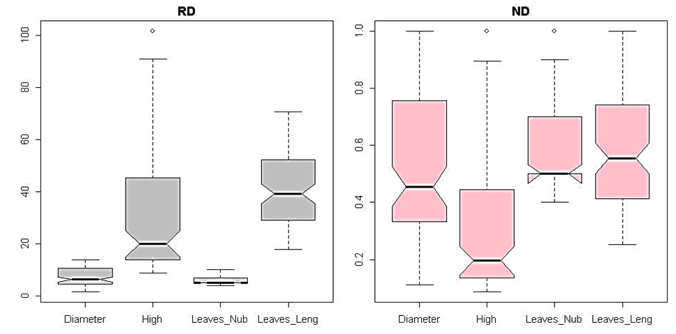Figure 1. Multivariate statistical analysis boxplot graphic in comparing row and normalized heterogenic data distribution for each considered parameter.

# Assessment of data normality by Shapiro-Wilk normality test for standardized and unstandardized data

Norm_Data=data.frame(w=shapiro.test(bio_data_matrix)$statistic,p=shapiro.test(bio_data_matrix)$p.value)

Row_Data=data.frame(w=shapiro.test(bio.data.matrix)$statistic,p=shapiro.test(bio.data.matrix)$p.value)

W<-rbind(Norm_Data,Row_Data)

write.table(W, file = "results/Shapiro.text.txt", sep = "\t")

Table 2. Result of Shapiro Wilk normality test for row data

Data standardization procedure seem to induce an apparent data normal distribution as oppose to row data distribution (p row data << p standardized data). However, in the present example, both row and standardized data don’t.

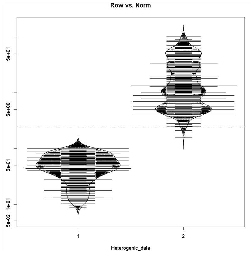Figure 2. Bean-plot graphic in comparing (1) row and (2) standardized data dispersion and/or distribution by merging processed variables data

Follow a normal distribution, since the p-value referred to these data normal distribution <<0.05 (Figure 3).

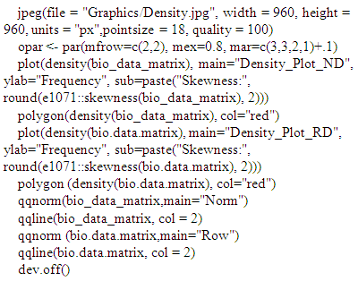
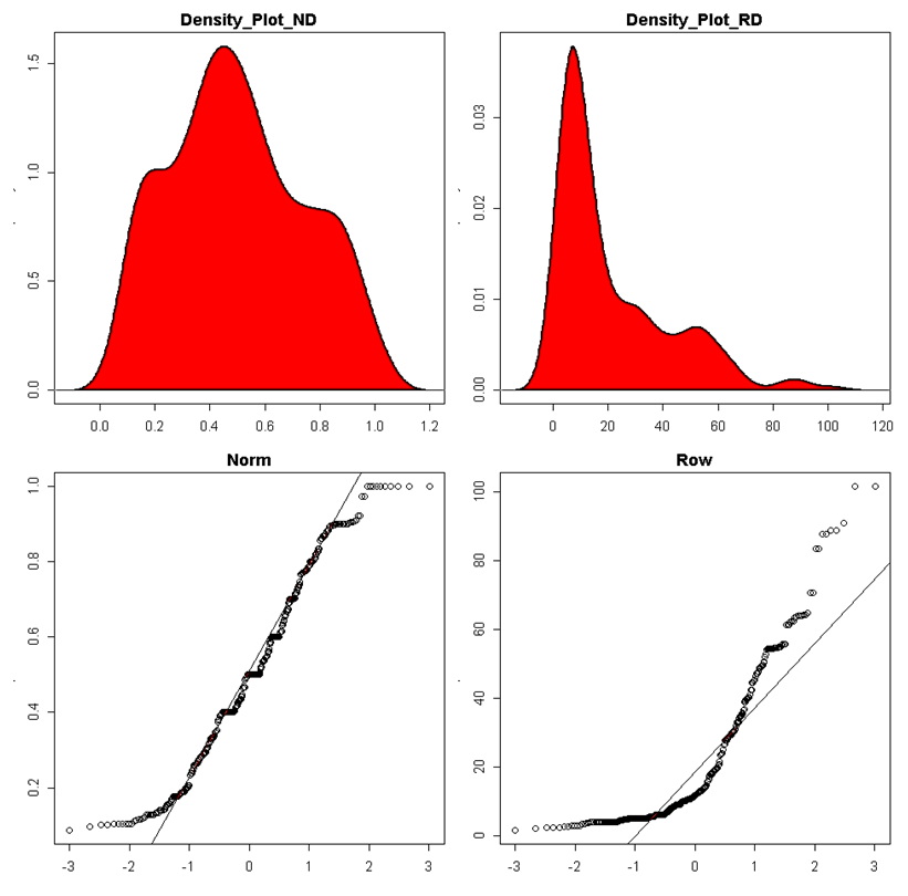Figure 3. Assessment of processed data (row and standardized/normalized data) normality by density plot and as well quantile normalisation methods

# Assessment of data normality by Shapiro-Wilk normality test graphical representation

# Pvcluster clustering survey

# Normalized and /or standardized data

result_ND <- pvclust(bio_data_matrix, method.dist="cor", method.hclust="average")

# Row and/or unstandardized data

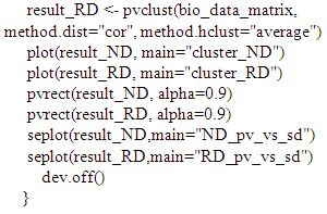
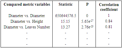
3.2. Correlation Test Analysing the Relationship between Paired Compared Metric Variables

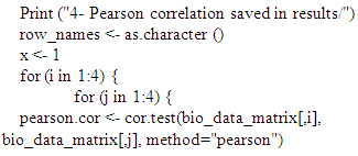
The pipeline provides both Pearson and Spearman correlation analysis. Here, users are also free in choosing correlation methods fitting better their analysis (pipeline flexibility).

# Correlation test and Pearson correlation matrix heatmap

cor_matrix <- matrix (nrow=16, ncol=3)

colnames(cor_matrix) <- c("statistic", "p.value", "correlation")

head_name <- c ("Diametre_cm", "Hauteur_cm", "Nb_de_feuilles", "Longueur_feuille")

# Pearson Correlation with variable couples table.

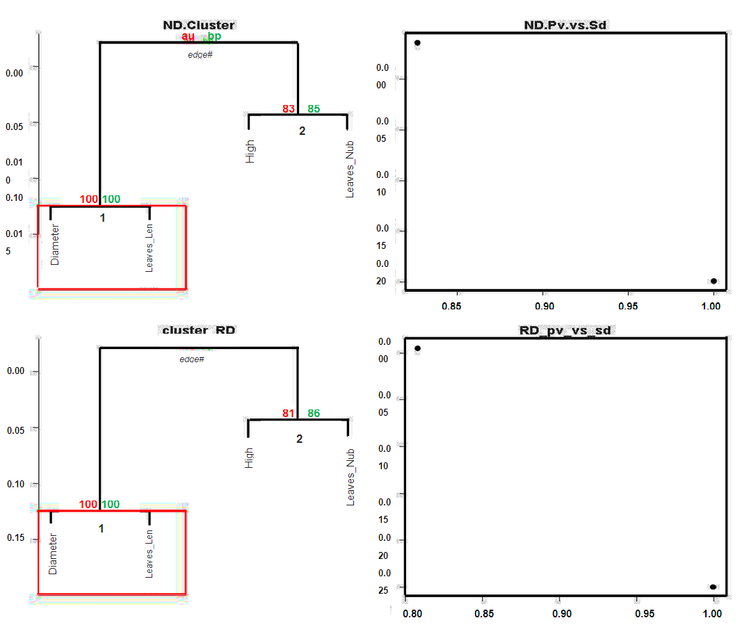Figure 4. R pvclust clustering survey providing two types of p-values; AU (Approximately unbiased) p-value and BP (Bootstrap probability); cluster dendrogram with AU/BP values (%) and (C and D): p-value vs. standard error plot analyzing paired analyzed features. ND: normalized data; RD: row data

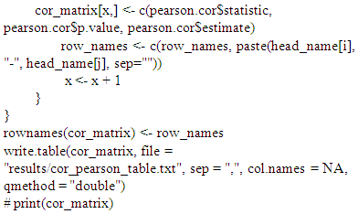# Spearman Correlation with variable couples table.

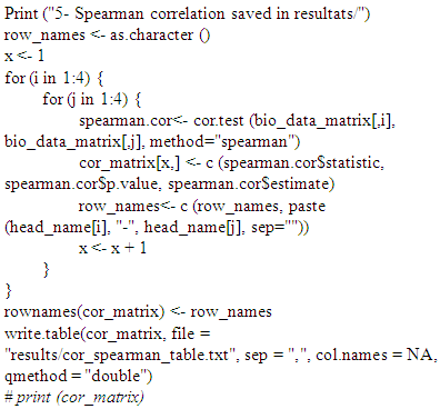#Heatmap Correlation

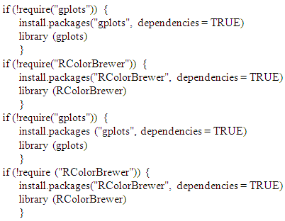#Correlation (Pearson and/or Spearman) Heatmap Graphic

Flexibility of our pipeline allows user to set and/or to use correlation method fitting better to their data. Here, we represented both Spearman and Pearson correlation heatmap for standardized data (ND). However, our pipeline provides correlation heatmap graphics for unstandardized data (RD).

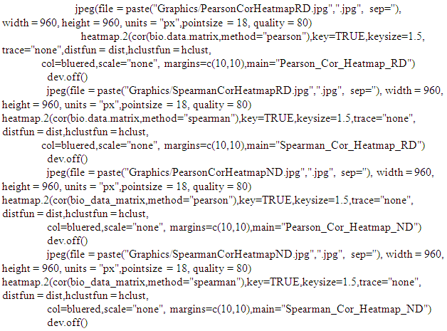
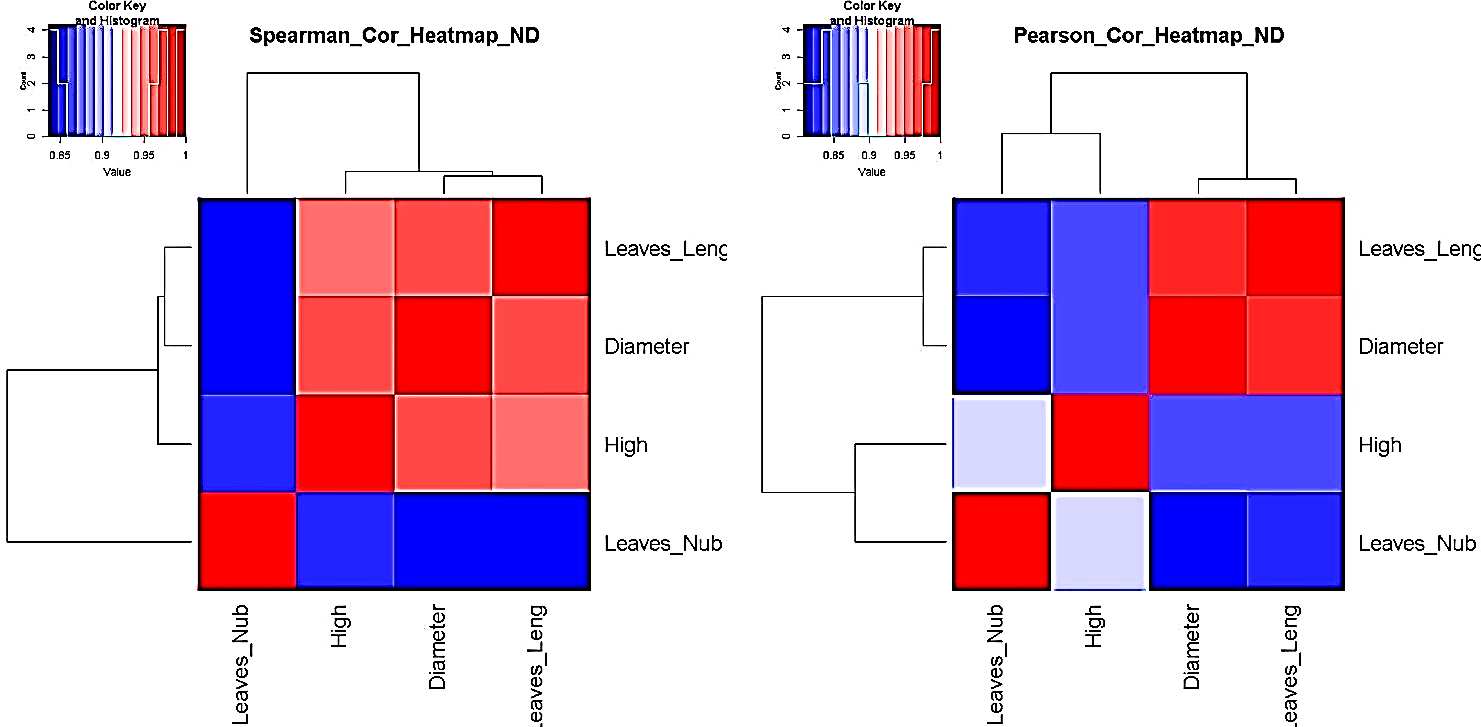Figure 5. i.e. Pearson and/or Spearman correlation heatmap survey in processing standardized (ND) pair metric variable parameters

The pipeline provides in the results folder complete comparison table with regard Pearson correlation test as well as Spearman correlation survey between all paired parameters. Here, we provided, just the head of the Pearson correlation test results (Table 3).

Table 3. Table header of Pearson correlation test provided by the pipeline by assessing the relationship between paired compared metric variables

3.3. Principal Component Analysis Assessing Processed Data Variance and Needed Factors for Explaining Metric Data Variability

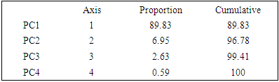
PCA survey is stabilized by processed data normal distribution (at least symmetrical). A prior data transformation can greatly help to improve the situation (our pipeline provide data standardization procedure). Also, data standardization is sturdily recommended before PCA analysis since giving the same weight to all the variables, and interprets the results in terms of correlation which is often easier.

bio_data_pca = princomp(bio_data_matrix)

jpeg(file = "Graphics/screeplot_barplot.jpg", width = 960, height = 960, units = "px", pointsize = 18, quality = 100)

screeplot(bio_data_pca, type = "barplot")

dev.off()

jpeg(file = "Graphics/screeplot_lines.jpg", width = 960, height = 960, units = "px", pointsize = 18, quality = 100)

screeplot(bio_data_pca, type="lines")

dev.off()

# Assessment of PCA survey quality

To estimate the quality of the analysis, we were interested in the percentage of variance explained by each axis. To obtain these percentages, developed pipeline assess Eigenvalues, and their contribution to the variance.

# Cumulative variance proportion

ACP<-rda(bio_data_matrix)

write.table(MVA.synt(ACP)[[1]]$tab,file="results/pca_variance.txt",sep="\t")

summary (ACP) function # provides detailed information with regard each analysed component by processing each factor and/or variable features.

# PCA Analysis quality control: graphic comparing observed data to estimated data for PCA survey

It may happen that the percentages of variance explained by the PCA are relatively small. This does not necessarily mean that the analysis is useless. Indeed, what matters is that the inter-individual distances in the multivariate environment created by the analysis (PCA) are well representative of the real and/or observed inter-individual distances (i.e. in the data table). To verify this, the pipeline draw a diagram of Shepard.

Jpeg (file = "Graphics/obs.val_vs_theo.val.jpg")

stressplot (ACP)

dev.off () # Shepard graphic was obtained by default by processing the first two axis (k=2; see Figure 7).

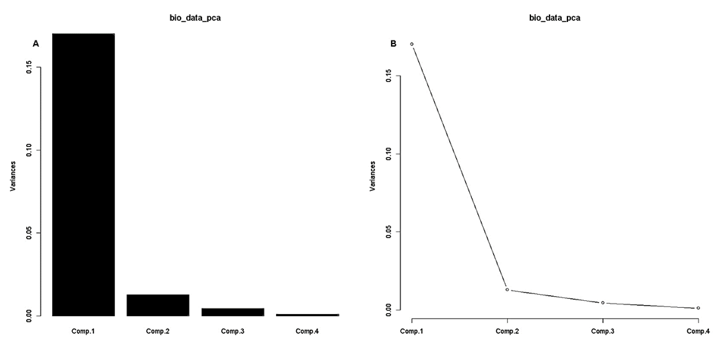Figure 6. Variance analysis via principal component analysis (PCA) of process metric parameters by (A) bar and (B) line scree-plot graphics

Table 4. PCA survey in assessing percentage of variance explained by each axis

# We assessed all components in summarizing observed and stimulated and/or theoretical data.

jpeg (file = "Graphics/all_obs.val_vs_theo.val.jpg")

opar <- par (mfrow=c(2,2), mex=0.8, mar=c(3,3,2,1)+.1)

stressplot(ACP,k=1) # k represents analyzed variables number. In our example four variables have been analyzed (see appendix table).

stressplot(ACP,k=2)

stressplot (ACP,k=3)

stressplot (ACP,k=4)

dev.off ()

On this diagram (Figure 7), if dots are roughly aligned along a straight line then the distances in the PCA environment are well proportional to the real observed distances guarantying a correct interpretation with regard analysis results. If dots clearly do not draw a line, the distances are not preserved. Results interpretation does not represent the reality.

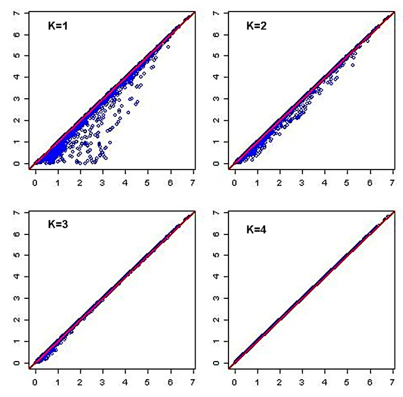Figure 7. Diagram of Shepard evaluating inter-individual distances in the multivariate environment created by PCA survey vs. observed inter-individual distances for standardized data

# Individual data dispersion vs. analyzed variables parameters correlation

jpeg (file = "Graphics/cor_cercle.jpg")

opar<-par (mfrow=c(2,2), mex=0.8, mar=c (2,2,2,1)+.1)

MVA.plot (ACP)

MVA.corplot (ACP)

dev.off ()

# Factor extraction for PCA survey

A crucial decision in exploratory factor analysis is how many factors to extract. Parallel analysis in principal component analysis survey is a useful method to established the number of principal component needed in a multi-variant statistical analysis in which theoretical estimate variance is computed and compared to observed (real variance) or experimental data (Dago et al, 2016). We provide parallel PCA analysis by using R “paran” package (R Equastat, 2016). Results highlighted needed factor(s) and /or number of passed component(s) in explaining process metric data variability by providing a table (Table 5) and as well a figure (Figure 9) indicating number of component(s) passed. Factor analysis is a statistical method used to describe variability among observed, correlated variables in terms of a potentially lower number of unobserved variables called factors. The observed variables are modelled as linear combinations of the potential factors. The information gained about the interdependencies between observed variables can be used later to reduce the set of variables in a dataset. Factor analysis and principal component analysis (PCA) methods have the aim of reducing the dimensionality of a vector of presently processed metric variables. Also both methods assume that the modelling subspace is linear. But while Factor analysis assumes a model, PCA is just a data transformation and for this reason it always exists. Furthermore, while Factor Analysis aims at explaining co-variances or correlations (Figure 9B), PCA concentrates on variances (Figure 9A).

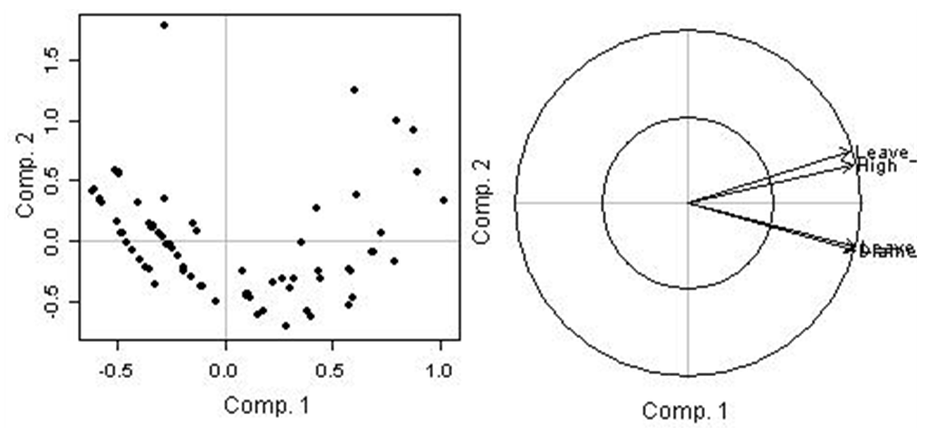Figure 8. Individual and variables circle correlation and/or inter-action graphics in assessing individual data variability.

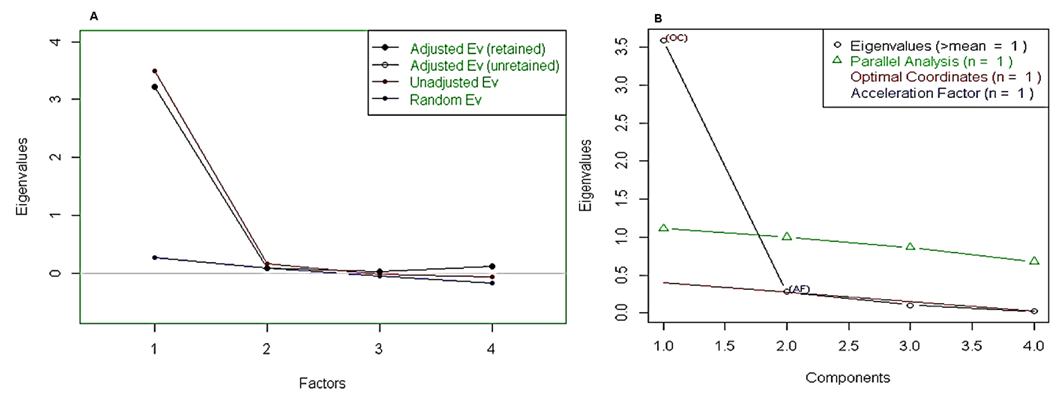Figure 9. Retained adjusted Eigenvalue vs. unadjusted Eigenvalue as well as estimated bias representation

Table 5 suggested that an adjusted eigenvalues > 0, indicated 4 factors dimensions to be retain, while an adjusted eigenvalues > 1 indicated factor dimensions to be retain (Figure 7A). Several typologies of analysis can be perform with the present processed PCA and n factor analysis.

Table 5. Results of Horn's Parallel Analysis for factor retention 5000 iterations, using the mean estimate

# Principal component analysis test of the hypothesis of number of needed factor in explaining data variability.

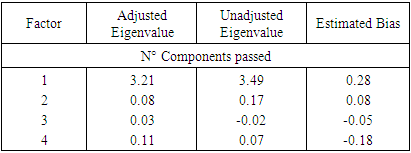
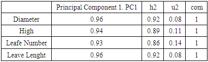
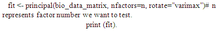The principal () function in the psych package can be used to extract and rotate principal components. Analyzed data can be a raw data matrix (i.e. bio_data_matrix, see additional file) or a covariance matrix. Pairwise deletion of missing data is used rotate can "none", "varimax" (see script above), "quatimax", "promax", "oblimin", "simplimax", or "cluster".

Here, we performed an example by processing test of the hypothesis for n=1, because of PCA n factor survey results that discriminated n=1 as optimal factor for explaining metric data variability (Figure 7B).

Test of the hypothesis that 1 component is sufficient exhibited the following results: root mean square of the residuals (RMSR) =0.06, with the empirical chi square = 4.34 with p< 0.11. The results of the present PCA factor analysis computing cumulative proportion with regard n=1 component in explaining metric data variability have been reported in Table 6. Also, principal component analysis provided communality (h2) and specific (u2) variance. Considering as a whole, proportion variance computed by PC1 =0.9.

Table 6. Test of hypothesis that n factor is sufficient explaining metric data variability

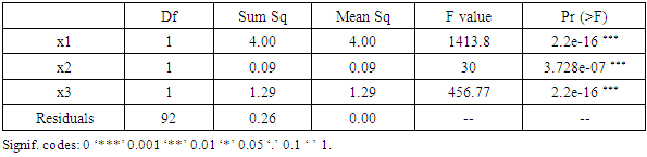
3.4. Anova and Multiple Linear Regression (MLR) Survey/Model by Linking Process Metric Variable Factors

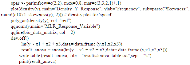
In our analysis we retrieved i.e. y as a response variable, while x1, x2 and x3 are explicative variables. The pipeline allows users to choose MLR variables, depending on their analysis.

y=(as.vector(bio_data_matrix[,1]))

x1=as.vector(bio_data_matrix[,2])

x2=as.vector(bio_data_matrix[,3])

x3=as.vector(bio_data_matrix[,4])

Before applying anova multiple linear regression survey, we assessed the normality of MLR response parameter (y).

jpeg(file = "Graphics/DensityResponse.jpg", width = 960, height = 960, units = "px",pointsize = 18, quality = 100)

Table 7. Anova results

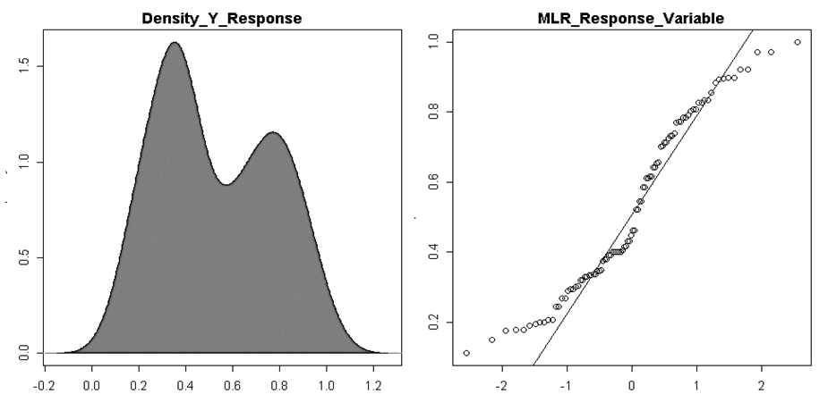Figure 10. Assessment of multiple linear regression response parameter (y) normality by density plot and as well quantile normalisation methods

4. Conclusions

The present study provides a semi-automatic computational bio-statistical pipeline for heterogenic agronomic metric data analysis in R programing environment. It noteworthy to underline that above mentioned pipeline has been wholly and/or partially used in processing several data typology analysis [17, 18, 31, 32, 33, 34 and 35]. Also, we believe that this platform will be helpful for researchers with weak programming skill in their early statistical survey. The pipeline offers multivariate descriptive as well as analytical approaches by providing tables and as well elaborate graphics with the purpose to help researchers in improving data statistical approach and as well interpretation. However, because of pipeline flexibility, we suggest and encourage users for integrating own statistical knowledge and/or approach if any.

Appendix

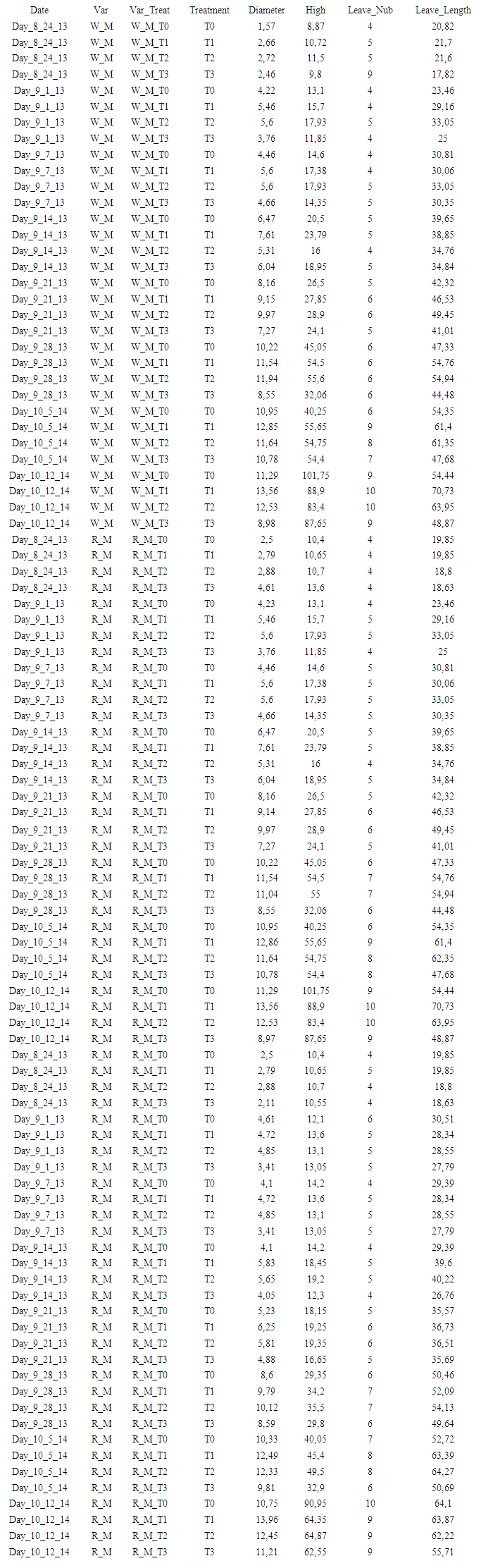Appendix 1. illustrative row matrix data processed by presently developed semi-automatic computational statistical pipeline

Appendix 2. Frame work of semi-automatic computational statistic pipeline functions and/or scripts