1. Introduction

DNA microarray technology enables the biologists to monitor expression levels of thousands of genes in a single microarray experiment. There is a high demand of computational techniques to operate on the massive amount of expression data generated by DNA microarray technology to extract important biological information. Due to the large number of genes and complex gene regulation networks, clustering is a useful exploratory technique for analyzing such data. It groups data of interest into a number of relatively homogeneous groups or clusters where the intra-group object similarity is minimized and the inter-group object dissimilarity is maximized. Problems of automatically classifying data arise in many areas, and hierarchical clustering can be a very good approach in certain areas such as gene expression data analysis because it can present a hierarchical organization of the clusters.

Extracting important biological knowledge from biological data is a difficult task. One very useful approach for providing insight into the gene expression data is to organize the genes in a hierarchy of classes, where genes in a class are more similar compared to its ancestor classes in the hierarchy. In this paper, we present a polythetic divisive hierarchical clustering algorithm that operates in two distinct steps. The first step generates a number of initial clusters and in the second step, these initial clusters are further processed to form a set of finer clusters. The algorithm advances clustering of microarray data in following ways (a) Extraction of initial clusters is faster and it does not require any proximity measure. (b) During discovery of final clusters, a proximity measure referred here as MRD(Mean Residue Distance) is used to find mutual distance among genes within a particular initial cluster instead of operating on the entire set. (c) The algorithm is capable of tuning the threshold to be used to decompose a node to its child nodes itself. (d) The algorithm stores the tree structure which can be later used in different applications. (e) The algorithm allows overlapping of genes among child nodes of a particular node.

The rest of the paper is organized as follows. In section 2, we discuss related work. Section 3 presents the algorithm. Experimental results are reported in section 4. Finally, discussion and future work are reported in section 5 and section 6 respectively.

2. Related Work

Hierarchical clustering usually generates a hierarchy of nested clusters or, in other words, a tree of clusters, also known as a dendrogram. Hierarchical clustering methods are categorized into agglomerative (bottom-up) and divisive (top-down). A large number of clustering techniques have been reported for analyzing gene expression data, such as Unweighted Pair Group Method with Arithmetic Mean (UPGMA)[1], Self Organizing Tree Algorithm (SOTA)[2], Divisive Correlation Clustering Algorithm (DCCA)[3], Density-Based Hierarchical clustering method (DHC)[4] and Dynamically Growing Self-Organizing Tree (DGSOT)[5]. Unweighted Pair Group Method with Arithmetic Mean adopts an agglomerative method to graphically represent the clustered dataset. The method is much favored by many biologists and has become one of the most widely-used tools in gene expression data analysis. However, it suffers from lack of robustness, i.e., a small perturbation of the dataset may greatly change the structure of the hierarchical dendrogram. DHC is a popular density based clustering algorithm. DHC is developed based on ‘density’ and ‘attraction’ of data objects. In the first level, an attraction tree is constructed to represent the relationship between the data objects in the dense area which is later summarized to a density tree. Another approach splits the genes through a divisive approach, called the Deterministic-Annealing Algorithm (DAA)[6]. Hierarchical clustering not only groups together genes with similar expression patterns but also provides a natural way to graphically represent the dataset allowing a thorough inspection. However, like UPGMA, a small change in the dataset may greatly affect the hierarchical dendrogram structure. Another drawback is its high computational complexity and vagueness of termination criteria.

Table 1. Some existing hierarchical clustering techniques Technique Approach ProximityMeasure InputParameters UPGMA Agglomerative Euclidean /Pearson'scorrelation cut-off forthedendrogram DGSOT Divisive,Model-based Any Heterogeneity threshold, Clusterseparationthreshold SOTA Divisive Any Heterogeneity threshold,Distancevalue threshold DHC Divisive, Density Based Pearson'scorrelation Radius similaritythreshold,minimum number of objects

Based on our selected survey, we have observed that most of hierarchical algorithms focus on the final clusters. Biologists are not only interested in the clusters of genes, but also in the relationships (i.e. closeness) among the clusters and their sub-clusters, and the relationship among the genes within a cluster. A clustering algorithm, which also provides some graphical representation of the cluster structure, is much favored by the biologists. To address this issue, this paper presents a hierarchical clustering algorithm GERC that generates a tree along with the set of clusters.

3. The GERC Algorithm

GERC is a polythetic divisive hierarchical clustering algorithm that operates in two distinct steps. This is an extended version of the article[7] where the method was introduced. In the first step of the algorithm, an initial cluster is formed and this initial cluster is further processed in the second step to form finer clusters. The algorithm accepts four input parameters i.e., reference gene, step down ratio, preferred node volume and MRD threshold. However, the last three parameters can be statistically computed from the expression data. The technique can operate on any high dimensional numeric domain.

3.1. Data Pre-processing

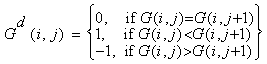
Often gene data available on the web are found to contain missing values. The quality of clusters largely depends on the handling of these missing values. Apart from missing value handling, pre-processing also involves normalization and discretization.

Handling missing values

We used the Local Least Squares Imputation method[8] to compute missing values in the datasets. There are two steps in the local least squares imputation method. The first step is to select k genes by Pearson correlation coefficient. The second step is regression using the selected k genes to estimate the missing values.

Normalization

The datasets are normalized using a common statistical method that converts each gene to a normal distribution with mean 0 and variance 1. This statistical method of normalization is often termed as Z score normalization[9] or Mean 0 Standard Deviation 1 normalization.

Discretization

The normalized matrix is discretized to a matrix by comparing a value in a column with the value in the next column of the same row. The normalized matrix consists of three discrete values 1 (if the next value is larger) , -1 (if the next value is smaller) and 0 (if the next value is equal). The normalized matrix G can be converted to the discretized matrix G^d in the following manner.

3.2. Proximity Measure

In this paper, we introduce a simplified form of mean squared residue measure, i.e., Mean Residue Distance(MRD) to find mutual distance of two genes that aids in extracting the coherent patterns in the expression matrix. Like mean squared residue measure, MRD is a measure that works satisfactorily to detect coherence of constant valued genes, constant row genes, constant column genes and additive genes. The significance of these correlations in clustering of gene expression data is reported in[10]. Unlike MSR, MRD can operate in mutual mode i.e., it can compute correlation between a pair of genes. Next we discuss the mean squared residue measure and then introduce MRD measure.

Mean Squared Residue

Mean squared residue is a measure that was used to find coherent objects in a data matrix by[11]. They tried to find out a subset of genes along with a subset of conditions which has mean squared residue less than a threshold δ. They termed such subspace clusters as δ biclusters.The measure is still considered a strong one to detect coherent objects if it is used carefully. Various subspace clustering algorithms use mean squared residue directly or with a bit of modification. Mean squared residue of an element a_ij in gene expression matrix is given by,

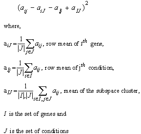Mean squared residue of a subspace cluster is computed as,

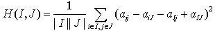
Figure 1. Visual interpretation of Mean Squared Residueo

Fig. 1 presents visual interpretation of MSR for two gene expressions g1 and g2. From the visual interpretation, it can be clearly stated that the measure can be effectively used to find mutual distance between two genes under a defined set of conditions. The proposed MRD measure is based on this fact. However, considering the cost effectiveness without deteriorating the cluster quality we simplify this measure by replacing the squaring operation with a modulus or absolute operation. Apart from this, the proposed measure is used in extracting finer subspace clusters from the initial subspace cluster in step 2 of the proposed algorithm.

Mean Residue Distance

The mean residue distance of an element a_i of gene g₁=( a₁, a₂,..., a_n) with respect to another element b_i of gene g₂=(b₁, b₂,..., b_n) is defined as,

Where a_mean is the mean of all the elements of g₁ and b_mean is the mean of all the elements of g₂. MRD of the gene pair g₁ and g₂ with respect to a subspace of conditions λ can be computes as,

Following definitions and theorems provide the theoretical basis and soundness of the proposed measure based on [12].

Definition 1: Coherent genes: Two genes are called coherent if similarity between the two genes is more than a given threshold in terms of a particular proximity measure.

Definition 2: Expression pattern: The expression pattern of a gene is defined as the discretized form of the gene expression values. Two genes are said to have similar expression pattern if their discretized values are same. Mathematically, two genes g_i and g_j have similar expression pattern if

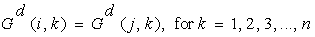Where n is the total number of conditions.

Definition 3: Constant valued genes: For two genes g_i=(a₁, a₂,...., a_n) and g_j=(b₁, b₂,..., b_n) if a₁=a₂=...=a_n=b₁=b₂=...=b_n, then the genes are called constant valued genes.

Definition 4: Constant row genes: For two genes g_i=(a₁, a₂,...., a_n) and g_j=(b₁, b₂,..., b_n), if a₁=a₂=...=a_n and b₁=b₂=...=b_n, then the genes are called constant row genes.

Definition 5: Constant column genes: For two genes g_i=(a₁, a₂,..., a_n) and g_j=(b₁, b₂,..., b_n), if a₁=b₁, a₂=b₂, ..., a_n=b_n, then the genes are called constant column genes.

Definition 6: Additive genes: For two genes g_i=(a₁, a₂,...,a_n) and g_j=(b₁, b₂,...,b_n) if b₁=a₁+d, b₂=a₂+d, ..., b_n=a_n+d, where d is an additive constant, then the genes are called additive genes.

Properties of MRD

The MRD measure is capable of detecting four types of coherence (a) Coherence among constant valued genes (b) Coherence among constant row genes (c) Coherence among constant column genes (d) Coherence among additive genes. Next we present some of the properties of MRD.

Theorem 1. MRD of two constant valued genes is always zero.Proof:

Let the two genes be g₁=(a₁, a₂,..., a_n) and g₂=(b₁,b₂,..., b_n). Since the two genes are constant valued so

a₁=a₂=...=a_n=b₁=b₂=...=b_n=x (say).

Now mean of the two genes will be, a_mean=b_mean=x.

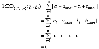Theorem 2. MRD of two constant row genes is always zero.

Proof:

Let the two genes be g₁=(a₁, a₂,..., a_n) and g₂=(b₁,b₂,..., b_n). Since these are constant row genes, so a₁=a₂=a₃=...=a_n=x (say) and b₁=b₂=b₃=...=b_n=y (say).

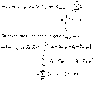Theorem 3. MRD of two constant column genes is always zero.

Proof:

Let the two genes be g₁=(a₁, a₂,..., a_n) and g₂=(b₁,b₂,..., b_n). Since these are constant column genes, so a₁=b₁, a₂=b₂,..., a_n=b_n.

Now mean of two genes will be a_mean=b_mean=m(say).

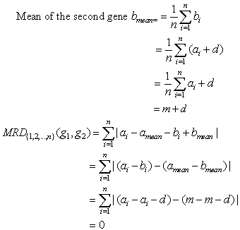
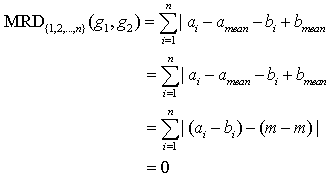Theorem 4. MRD of two additive genes is always zero.

Proof:

Let the two genes be g₁=(a₁, a₂,..., a_n) and g₂=(b₁,b₂,..., b_n). Since the genes are additive, so b_i=a_i+d, for i=1,2,3,...,n. Here d is an additive constant.

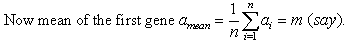
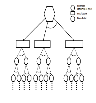Figure 2. Structure of GERC tree

3.3. GERC Tree

Our algorithm results a tree called GERC tree. The leaves of this tree present the generated clusters of the algorithm. This tree can be used to derive additional biological information from a gene expression dataset. The overall structure of the tree generated for more than one reference gene is presented in Fig. 2.

Dendrogram versus GERC tree

A dendrogram is binary tree that presents the hierarchical structure of the clusters generated by a hierarchical algorithm. In divisive hierarchical algorithm, dendrogram is obtained by recursively splitting a node containing a set of objects into two child nodes based on the similarity among the object pairs until all nodes have a single object. Conversely, in agglomerative approach, the nodes containing a single object are recursively merged until all the objects are in the root node. But in our algorithm, GERC tree is obtained by recursively splitting a single node containing the set of all objects into multiple nodes(with possibly common objects) until number of objects in all the processing nodes is less than or equal to a user given threshold, i.e. preferred node volume. Unlike Dendrogram, GERC tree is not a binary tree and the structure of the tree is flexible depending on the values of the set of input parameter. The structural difference between dendrogram and GERC tree is presented in Fig. 3.

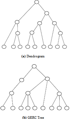Figure 3. Dendrogram versus GERC tree

Table 2. Comparison of Dendrogram VS GERC Tree Dendrogram GERC tree Tree Structure Binary General Overlapped objects in child nodes No Yes Tree structure depends on Input parameters Usually not Yes

Table 2 presents a general comparison of dendrogram and GERC tree. GERC tree conveys a more exhaustive set of information to the users. User can look for the nodes in the tree that is flourished in terms of their functional enrichment. Moreover, we can trace the path of a particular gene from the root node to the leaf nodes which may be useful to find its co-members in a particular functional category. This tree can also be useful to derive relationship in terms of their regulatory information such as co-regulation.

3.4. Proposed Algorithm: GERC

Following definitions, symbols and notations are used to describe the GERC algorithm.

Table 3. Symbolic representations SYMBOL MEANING Nc Total number of condtions Rg Reference gene n No of genes G The gene expression matrix Gd Discretized gene expression matrix gi ith gene T Preferred Node Volume C Initial Cluster η(i) ith node of the tree Nη Number of tree nodes dist(gi,gj) MRD between ith and jth genes as in the distance matrix α MRD threshold δ Step down ratio Neighbour β(gi) Neighbours of ith gene with respect to MRD threshold β Exp(gi) Expression pattern of ith gene presented by ith row of the discretized matrix father(η(j)) father of jth node degree β(gi) Degree of ith gene with respect to MRD threshold β η(j).threshold MRD threshold of jth tree node η(1) The root node of the GERC treecontaining all the genes

Definition 7: Neighbour: Two genes g_i and g_j are said to be neighbours of each other with respect to a threshold β if dist(g_i,g_j)≤β .

Definition 8: Degree: The degree of a gene g_j with respect to threshold β is defined as the number of genes which are within the β neighbourhood of g_j.

Definition 9: Initial Cluster: An initial cluster is defined as a subset of genes S such that for any two genes g_i, g_j in S, Exp(gi) =Exp(gi) in terms of at least (Nc/2)+1 numbers of conditions.

Definition 10: Finer Cluster: A finer cluster is defined as a set of genes S such that for any two genes gi, gj in S

ⅰ Exp(gi) = Exp(gi) in terms of (Nc/2)+1 numbers of conditions.

ⅱ dist(gi,gi)<= δ^l xα, where l is greater than or equal to the level of the node to which the finer cluster is associated.

The GERC algorithm consists of two steps. In the first step of GERC, all genes which have expression pattern similar to the reference gene in terms of (Nc/2)+1 number of conditions are put in an initial cluster. In the second step of the algorithm, the initial clusters are processed to produce finer clusters. While processing an initial cluster, all genes are put in the root node. Then iterative clustering is performed using a tuned MRD threshold on genes of each node to produce its child nodes. The process is repeated till all nodes in the tree contain a number of genes greater than user specified preferred node volume. The tuning of MRD threshold is governed by the user defined parameter step down ratio. The leaves of the tree represent the generated clusters. The algorithm can be used to produce a wide range of clusters by considering more than one reference gene. The detail of the algorithm is presented next.

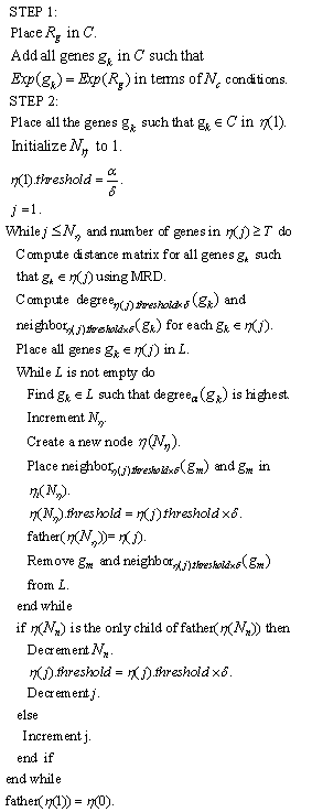In GERC, the reference gene is used as an input parameter. The algorithm tries to find the initial cluster to which this gene potentially belongs to. While finding this initial cluster it tries to locate all genes which have similar expression pattern with the reference gene in terms of at least (Nc/2)+1 number of conditions. If we want to explore the entire dataset we can use each of the available genes or a set of stochastically selected genes as reference genes. Once we discover the initial clusters we move to step 2 of the algorithm. In the second step, we create a single node first with all genes of the initial cluster in it and then iteratively cluster each node(having genes more than preferred volume umber of genes) of the tree until all the processing nodes in the tree have less than or equal to preferred volume number of genes. The input parameter step down ratio is actually used to reduce the value of MRD threshold as towards leaf nodes of the tree the similarity among genes increases and require a smaller value of MRD threshold. e.g. if the MRD threshold provided by user is 1 and step down ratio is .5, then the first node will use 1 as its MRD threshold while clustering. On successful division of the node to its children, the successive level nodes will use thresholds .5(1*.5),.25(.5*.5) …. and so on. Finally the sub-trees (one sub-tree in case of single reference gene) generated from the initial clusters are combined to form the GERC tree. The roots of these subtrees are made children of a single node that contains the set of entire genes and this node becomes the root of generated GERC tree.

3.5. Complexity Analysis

Since GERC involves two distinct steps, hence the total complexity is the sum of the complexities of these two steps. Let a dataset contains n number of genes. In the first step of the algorithm, the total number of comparisons done to put all n number of genes in the initial cluster is n-1. In the second step, if the number of genes in the initial cluster is p, the computation of distance matrix involves px(p-1)/2 operations. If the average number of genes in the non leaf nodes is m and the total number of non leaf nodes is l, creating the child nodes and hence the entire tree requires l*m operations. So complexity of the second step is O (px(p-1)/2+ l*m).

4. Experimental Results

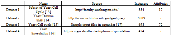
We implemented the GERC algorithm in MATLAB and tested it on four publicly available benchmark microarray datasets mentioned in Table 4. The test platform was a desktop PC with Intel Core 2 Duo 2.00 GHz processor and 512 MB memory running Windows XP operating system. Fig. 5, 6 and 7 present a part of the tree generated from an initial cluster for Dataset 2, Dataset 3 and Dataset 4 respectively.

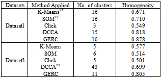
4.1. Cluster Quality

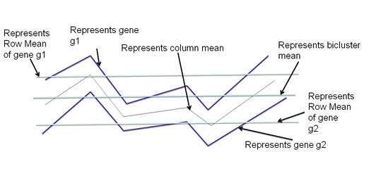
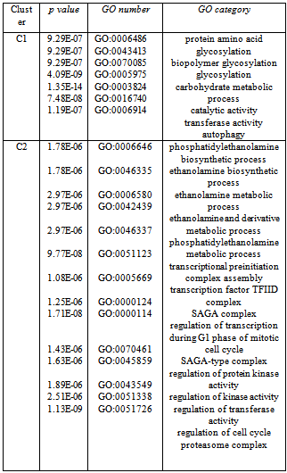
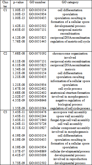
The GERC algorithm was compared with various clustering algorithms and the results were validated using average homogeneity score[18], p value[19] and z score[20].

Cluster Homogeneity: Homogeneity measures the quality of clusters on the basis of the definition of a cluster i.e., Objects within a cluster are similar while objects in different clusters are dissimilar. It is calculated as follows.

(a) Compute average value of similarity between each gene g_i and the centroid of the cluster to which it has been assigned.

(b) Calculate average homogeneity for the clustering C weighted according to the size of the clusters.

Table 4. Datasets used for experimental results

The homogeneity values for the GERC algorithm and some other algorithms are reported in Table 5. It can be observed that the homogeneity value for GERC is highest from which we can conclude that the coherence of the clusters produced by GERC are better than those produced by competing algorithms.

p value:The biological relevance of a cluster can be verified based on the gene ontology (GO) annotation databasehttp://db.yeastgenome.org/cgi-bin/GO/-goTermFinder. It is used to test the functional enrichment of a group of genes in terms of three structured controlled ontologies, viz., associated biological processes, molecular functions and biological components. The functional enrichment of each GO category in each of the clusters obtained is calculated by its p-value.

The p-value is computed using a cumulative hyper geometric distribution. It measures the probability of finding the number of genes involved in a given GO term (i.e., function, process and component) within a cluster. The genes in a cluster are evaluated for the statistical significance by computing the p-value for each GO category. This signifies how well the genes in the cluster match with different GO categories. The p-value represents the probability of observing the number of genes from a specific GO functional category within each cluster. A low p-value indicates the genes belonging to the enriched functional categories are biologically significant in the corresponding clusters.

To compute p-value, we used the software FuncAssociate[19]. FuncAssociate computes hyper geometric functional enrichment score based on Molecular Function and Biological Process annotations. The enriched functional categories for some of the clusters obtained by GERC on Datasets 1, 2 and 4 are listed in Tables 6, 7 and 8 respectively. The functional enrichment of each GO category in each of the clusters is calculated by its p-value. To restrict the size of the article we have reported p-values of only three clusters. The clusters contain the highly enriched cellular components of DNA metabolic process, DNA replication, chromosome, chromosomal part, cell cycle, sporulation, cell differentiation, developmental process, meiosis cellular component assembly involved in morphogenesis, catalytic activity, carbohydrate metabolic process etc with p-values of 1.67x 10^-11 , 2.34 x 10^-12 , 1.49x 10^-5 , 1.98 x10^-12 , 1.12x10^-10 , 1.00x 10^-13 , 1.00 x 10^-13 , 1.42 x 10^-11 , 1.54x10^-16 , 8.31x 10^-12 , 1.35x10^-14 and 4.09 x10^-09 , respectively. From the Tables, we can conclude that GERC shows a good enrichment of functional categories and therefore projects a good biological significance.

Table 5. Homogeneity values for GERC and other comparable algorithms

Table 6. P-value of some of the finer clusters for Dataset 1

Table 7. p-value of some of the finer clusters for Dataset 2

z-score: We used Gibbons ClusterJudge[20] tool to calculate the z-score. A higher value of z-score indicates that genes are better clustered by function, indicating a more biologically relevant clustering result. Table 10 presents generated average z-score of GERC along with some other clustering algorithm. From the results it can be observed that GERC performed satisfactorily compared to the other algorithms in terms of z-score.

5. Discussion

We have presented here a clustering algorithm that generates a tree where the children of a node represent the clusters that are formed from the genes in that node. The leaf nodes of the tree will represent the desired clusters. We keep on reducing the threshold used in the clustering process as we move on to deeper levels. The structure of the generated tree is driven by the input parameters. The input parameters T and δ controls the height/depth of the tree. If we set the value of T large the genes in the root node will split to the leaf nodes in a few numbers of levels.

Table 8. p-value of some of the finer clusters for Dataset 4

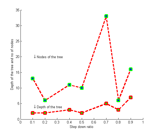Figure 4. Tuning the value of δ for Dataset 3

If we set the value of δ small, it will lead to fewer levels as the difference between the thresholds used in the subsequent levels will become larger. α (MRD threshold) should be carefully chosen. A small value of α may leave out some upper levels of the hierarchical tree. The effect of these parameters on the tree structure is presented in Table 9. To decide the value of δ, we drew two graphs (Fig. 4), one for number of nodes and another one for depth of the sub tree generated from an initial cluster against different values of δ. We used a trade off between these two graphs and decided to use 0.7 as the value of δ for yeast cell cycle dataset.

Table 9. Effect of Input Parameters ∂ α T No of nodes Depth 0.4 2 10 11 3 0.9 2 10 16 7 0.7 2 3 33 5 0.7 2 12 7 2

6. Conclusions and Future Work

In this paper, we present a top down hierarchical clustering algorithm that produces a tree of genes in the neighbourhood of a reference gene called GERC tree along with the generated clusters. The algorithm can be used to generate a wide range of clusters by considering multiple reference genes. Clustering performed in the nodes at different levels of GERC tree adaptively chooses the values of threshold parameters. The complexity of our approach can be improved by using an appropriate heuristic method for estimating an effective set of parameter values which will guarantee for quality cluster results. The value of α and R can also be calculated statistically from the set of input genes. Work is underway for integrating prior biological information to the clustering process to improve the results.

Table 10. z-scores for AMC and some counterparts for Dataset 2 Methiod Applied z-score K means[16] 5.57 SOM[17] 5.78 DCCA[3] -0.78 GenClus[18] 7.39 AMC 7.35

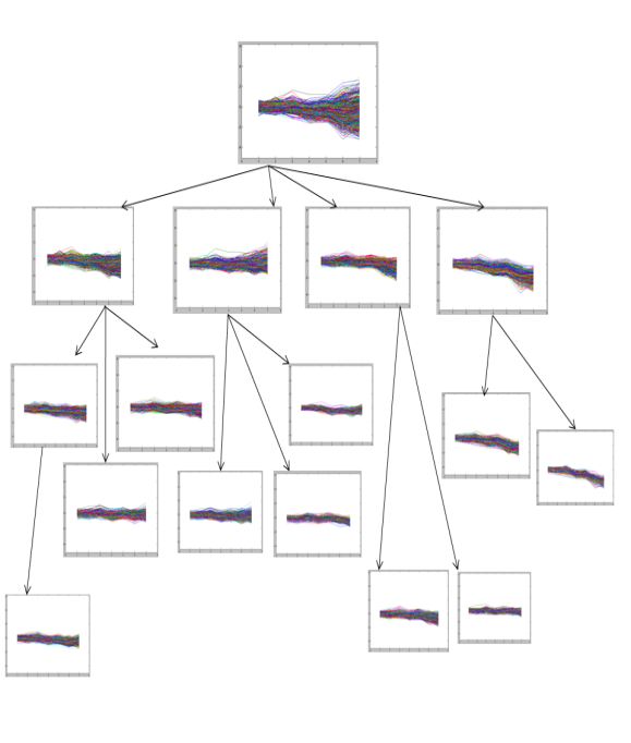Figure 5. Tree generated from an initial cluster for yeast Dataset 2

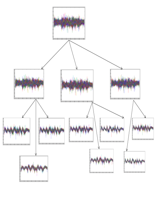Figure 6. Tree generated from an initial cluster for yeast Dataset 3

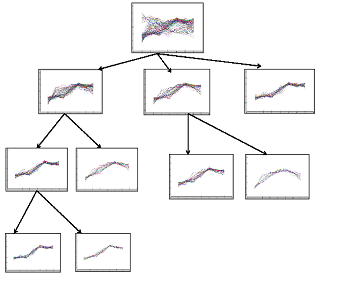Figure 7. Tree generated from an initial cluster for yeast Dataset 4

ACKNOWLEDGEMENTS

This work is an outcome of the research project in collaboration with CSIR, ISI, Kolkata funded by DST, Govt. of India. The work is also supported by INSPIRE programme of DST, Govt. Of India.