1. Introduction

Clustering is commonly used to reveal biological meaningful pattern in data arising from microarray experiment, which is called gene expression data. Further, it is the most common tool for interaction identification, as similar objects form a cluster. Clustering is unsupervised classification[1], also known as cluster analysis, which discovers grouping(s) of a set of patterns, objects or points. It is prevalent in any discipline that involves interaction identification. Unfortunately, clustering is difficult for most data sets due to its diverse shapes, densities, sizes and background noise. Gene expression data are usually arranged in a 2-dimensional matrix, where rows represent genes and columns represent samples or experimental conditions. Each element of this matrix represents the expression level of a gene under a specific condition, and is represented by a real number. In this case, genes that are similar may share a common biological pathway and the groupings of predictivegenes can be of interest to biologist. Conventional clus ter ing techniques are based on similarity between genes across all samples or experimental conditions. However, genes may be co regulated under some specific experimental conditions and shows weak similarity beyond these conditions. Therefore, a group of genes forms cluster under a subset of conditions. This technique of two-way clustering referred to as biclustering, in which both genes and conditions are clustered simultaneously.

2. Related Work

Several biclustering algorithms have been proposed in different application scenarios but we concentrate on graph theoretic approaches. In order to extract biclusters, these algorithms usually employ heuristic or probabilistic model. An illustrative discussion on many of these algorithms can be found in[4,5].

Cheng and Church[2] identify biclusters with the help of mean squared residue score, which is a measure of the coherence of rows and columns in the bicluster. Here the user has to input a value of mean residue score δ and the number of biclusters to be extracted. This method involve several iterations and each iteration produce only a single bicluster while previously identified biclusters are masked with random values. However they did not address the issue of noisy data, where as in this paper we concentrate on noisy data.

Tanay et al.[6] introduced SAMBA, in which the data are modelled as a bipartite graph with genes corresponding to vertices in one bipartition and samples corresponding to vertices in other bipartition, where edges representing significant changes in expression. Edges and non-edges are weighted by likelihood scores derived from a probabilistic model for the bipartite graph. A bicluster is defined as a heavy subgraph, where the weight of the subgraph is the sum of the weights of the corresponding edges and non-edges. It repeatedly finds the maximal highly-connected subgraph in the bipartite graph and performs local improvement by adding or deleting a single vertex until no further improvement is possible. In order to avoid exponential runtime, they assumed that row vertices have d-bounded degree. However, our technique can handle graphs of arbitrary degrees.

Ahsan and Amir[3] identify biclusters by recursively removing noise with the help of crossing minimization technique. This method is based on binary representation of the bipartite graph corresponding to input data matrix. It is difficult to produce coherent biclusters, as this method use a static discretization of the input data matrix.

Waseem and Asfaq[7] proposed cHawk, to identify biclusters with the help of crossing minimization paradigm. This method employs the barycenter heuristic to arrange vertices in both layers of a bipartite graph. The similarity test is done based on bregman divergence. This approach is similar to our approach as we also employ bipartite graph for representation of gene expression data. The time complexity of this technique is, where n and m are the number of rows and columns of the input data matrix and d is the average degree of overlap among biclusters, which is slower than our approach.

Wang and Liu[8] proposed RMSBE, which can identify optimal square biclusters with the maximum similarity score. This method performs multiple scans of the data matrix in order to compute similarity score, reference gene identification and bicluster identification. The time complexity of this technique is where n is number of rows and m is number of columns. Due to this cubic nature of complexity, it is not feasible for very high dimensional data.

Prelic et al.[9] proposed BiMax, which can identify constant biclusters. This method discretize the input expression matrix into a binary matrix based on a threshold value. Therefore it is difficult to identify coherent biclusters.

Bergmann et al.[10] proposed the iterative signature algorithm (ISA) that uses gene signatures and condition signatures in order to extract biclusters with both up and down-regulated expression values. They identify several transcription modules (biclusters) by executing the algorithm on reference gene sets. The reference gene sets needs to be carefully selected for extraction of good quality biclusters.

Zhao and Zaki[11] proposed Tricluster, for mining coherent clusters in 3-dimensional gene expression data sets. They construct a range multigraph and then searches for constrained maximal cliques in this multigraph, in order to extract a set of biclusters. However, they do not address the issue of noisy data, where as our approach can effectively handle noisy data.

3. Model Formulation

Let be a set of n genes and be a set of m experimental conditions. Microarray data-set is a real valued expression matrix where, and each entry corresponds to the logarithm of the relative abundance of mRNA of a gene under a specific experimental condition. A bicluster corresponds to a sub matrix that exhibits some coherent tendency. Let B be a sub matrix of dataset D i.e Bicluster where and, provided certain conditions of homogeneity are satisfied. We define the volume or size of a bicluster B as the number of elements, such that and. Let S be the set of all biclusters that satisfy the given homogeneity conditions, then is called a maximal bicluster iff there doesn’t exist another bicluster such that

Let be any arbitrary sub matrix of B.

B will be a valid bicluster iff it is a maximal bicluster satisfying the following conditions:

between two specified column values for a given row and be the weight of the row for this specified two column values.

Let us consider and be the weighted difference of two column values for a given row i and j respectively. We need that where is the multiple of maximum weight in the corresponding gene-set i.e

We also need that and , where and denote minimum cardinality thresholds for each dimension.

We consider an edge as valid, when the weighted difference range for a condition pair satisfies the threshold value so that it generates a gene-set. In order to produce large enough clusters, the minimum size constraints i.e , and are imposed. B is a scaling bicluster if and and where is a constant multiplicative factor. B is a shifting bicluster iff and and where is constant additive factor. B is a constant bicluster if or B is a constant row bicluster if or . Similarly B is a constant column bicluster if or, where is a typical value within the bicluster; and are adjustment for row and column respectively. B is overlap bicluster if is the sum or product of the contribution of different biclusters to which they belong.

Bipartite Graph: A graph is called Bipartite if its vertex set V can be decomposed into two disjoint subsets and (i.e. ) such that every edge in E joins a vertex in with a vertex in .

We consider weighted bipartite graph with where denotes the weight of the edge between vertices iand j.

3.1. Preprocessing

Gene expression data is usually noisy and may contain missing values. Illustrative discussion on prediction of missing value can be found in[12, 13]. Therefore it is essential to condition the data before applying the clustering algorithm. In order to handle missing values, we have adopted the approach used in[14] i.e. replacing all missing values by zero. Before normalizing the dataset, data beyond a threshold value (three standard deviation), has been temporarily removed to reduce the effect of outliers in the data. Then, the gene expression data is transformed using z-score standardization, where the transformed variables have a mean of 0 and variance of 1. Finally, the temporarily removed outliers that are below the mean value are replaced by the minimum value, where as the outliers above the mean values are replaced by the maximum value of the final normalized data. In order to handle outlier efficiently, we have partitioned the normalized condition data into unequal length intervals based on mean value. The motivation of considering unequal length intervals is due to the ineffectiveness of equal length intervals for extreme outlier values. Also the decision of number of intervals may lead to inappropriate interval boundaries, as it does not depend on the properties of data[15]. In this approach, we partition the condition column data into two halves with the mean value. Then, recursively each half is partitioned again into two halves with its own mean. This process proceeds until each condition column has been partitioned into required number of intervals. The number of intervals r for each condition depends on the data size n . Further, to have balanced partition, it is assumed that, where k is a positive integer and where 35 is the minimum sample size for large sample procedures[16]. The values within the intervals are then smoothed by interval means. We found that this way of partitioning is very effective and can deal with outliers efficiently.

3.2. Constructing Weighted Range Bipartite Graph

For a given dataset D, the minimum size threshold, and, and the maximum weighted difference threshold, let and be any two condition columns of D and let be the weighted difference of the expression values of gene in columns and such that, where. In order to incorporate the idea of mutual importance between two columns, we have computed the weight of all rows for specified column pairs. A difference range is defined as an interval of difference values , with. Let be the set of genes, whose difference w.r.t. columns and lie in the given weighted difference range. A difference range is called valid iff where is the multiple of maximum row weight in the corresponding gene set. Normally, for microarray experiment data, genes and conditions are represented by and vertex sets respectively, and the edge weight represents the response of gene to condition. However, in order to have a very compact representation, in this paper, we construct the weighted undirected bipartite graph by partitioning the condition set into two disjoint sets called upper layer and lower layer. The conditions that do not have any data values are not considered in the formation of disjoint sets. Here, each edge in the range bipartite graph has associated with it the rank and gene-set corresponding to the weighted difference range on that edge. Different bipartite graphs emerged for different threshold value, which is the multiple of maximum weight value in the corresponding gene-set. Consequently, we will have different types of biclusters. We have given priority to all valid edges that have large number of genes in the gene-set, by assigning rank to these edges. Ranks have been assigned on the basis of total number of genes in the gene-set i.e. The gene-sets having highest cardinality have been assigned rank 1, the second highest rank 2, the third highest rank 3 and so on. The inclusion and deletion of edges depends upon the value of and order in which we process these ranks and conditions. Let and be the set all valid edges and gene-sets respectively, in ascending order of rank values.

Table 1. Example of Microarray Dataset c0 c1 c2 c3 c4 g0 1 2 3 0 0 g1 0 0 0 4 5 g2 1 2 3 0 0 g3 0 0 0 4 5 g4 1 2 3 0 0

Figure 1. illustrates the steps for computing the weighted difference range for columns and in Table 1. Let, which is the maximum row weight in the gene-set, and considering then there is only one valid weighted difference range and the corresponding gene-set in sorted order is. Similarly, we compute weighted difference range for other experimental conditions. In this case, the number of valid ranges depends on the value of. For the sorted difference values, we find all valid weighted difference ranges for all pair of columns. Further, for simplicity, we have not considered rows with weight 0.

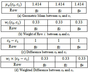Figure 1. Weighted difference range for c0 and c1

Here we may have overlapping of different ranges. The algorithm for partitioning condition set into and, for construction of bipartite graph is given in Algorithm I. From Table 1, a maximal weighted range bipartite graph is constructed (Figure 2). Let be the set of columns with missing value in each row. Let be the set of conditions such that. We have taken weight of the edge as rank for the corresponding gene-set. This algorithm gives priority to the edges having large rank in order to compensate the deletion of few valid edges, while partitioning the condition set into two disjoint sets. If there is a tie among rank values, then we randomly select an edge and start constructing the bipartite graph. As we deal with noisy data, additive and multiplicative methods of finding clusters may not always lead to good results. Therefore, instead of comparing two column values independently[11], we have computed weight of each row for any two specified column values. We build bipartite graph model of data, after properly conditioning the input data.

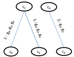Figure 2. Weighted Range Bipartite Graph G′

Algorithm I: Partitioning of Condition Set

Input:

Output: Creation of two disjoint sets and

Initialization:

1. while

2. for each valid edge do

3. if and then

4. insert and in

5. endif

6.if and then

7. insert and in

8. endif

9. endfor

10. endwhile

3.3. Experimental Setup

We have implemented our proposed algorithm in C++ under windows environment on a computer with configuration of Core 2 Duo 2.2 GHz of CPU and 3 GB RAM. The accuracy and performance of this algorithm is evaluated using synthetically generated dataset and real dataset. For synthetic data generation, a technique parallel to a methodology proposed in[9] is adopted whereas for real dataset, the model organism Yeast Saccharomyces Cerevisiae dataset is considered, since the yeast GO annotations are more extensive compared to other organisms. This dataset is provided by Gasch et al.[17], which contains 2,993 genes and 173 different stress conditions.

4. Bicluster Extraction and Evaluation

4.1 Bicluster Extraction

The weighted range bipartite graph is constructed by partitioning the set of experimental conditions into two disjoint sets and Each edge of this graph is associated with a rank value and the corresponding gene-set. The algorithm for extraction of biclusters from this graph by employing depth first search technique is given in Algorithm II. This algorithm requires the value of and the weighted bipartite graph as its input parameter. 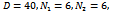The output of this algorithm is a set of biclusters and the number of such biclusters depends upon the dataset.

For example, let us consider the value of input parameters and. The algorithm starts searching the graph at a valid edge having highest rank value. In this case, it starts with the valid edge and get the corresponding reference cluster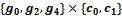. Then, other adjacent valid edges are explored that leads to the formation of final bicluster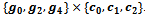. If a new edge does not have the sufficient number of genes and conditions, the reference bicluster is declared as the final bicluster, since this is maximal and satisfies all required conditions. Further, other valid edges are searched that leads to the formation of final bicluster. Here both the biclusters satisfies the minimum threshold value.

Algorithm II: Bicluster Extraction

Input:

Output: S

Initialization:

Call

1.

2. if then

3. if such that then

4. if then

5. remove

6.

7. endif

8. endif

9. endif

10. foreach do

11.

12.

13. forall edges do

14. if then

15.

16. endif

17. if then

18.

19. endif

20. endfor

21. endfor

22. Return S

4.2. Evaluation

For evaluation purpose, we need to compare our algorithm with other biclustering algorithms. As different biclustering algorithms deals with different problem formulations and clustering criteria, it is difficult to have a comparative study among such algorithms. Therefore, these algorithms work efficiently in certain situation and perform poorly in others. In view of this problem, we need to provide a common setting for such algorithms so that we can perform a fair comparative study. Our main focus lies on validating our proposed algorithm for extraction of constant, coherent and overlapped biclusters from noisy gene expression data with high accuracy in comparison to other similar algorithms. In view comparison, similar algorithms like CC[2], ISA[10], cHawk[7], SAMBA[6], RMSBE[8] and BiMax[9] are considered. We have used the Bicluster Analysis Toolbox (BicAT) developed by Prelic et al.[18] for implementation of BiMax, CC and ISA. Further, for implementation of SAMBA, EXPANDER developed by Maron-Katz et al.[19] is used and RMSBE implementation was downloaded from[20].

4.2.1. Complexity Analysis

Since we require to evaluate all pair of conditions, compute the weight of each gene, and find the weighted difference range to get the corresponding gene-set, the range bipartite graph construction step would take time. Here, we have considered the experimental conditions as vertices for the bipartite graph. These vertices are partitioned into two disjoint sets on the basis of rank of valid edges. This way of constructing bipartite graph leads to deletion of some valid edges and as a result, fewer edges need to be processed in comparison to other graph approach for solving the same problem. Therefore, the running time can be significantly reduced for this representation of gene expression data using a bipartite graph. The bicluster extraction step depends on the value of input parameters and datasets. This step is most expensive as there can be exponential number of clusters. Since the experimental conditions are only considered as vertices, and some uninteresting edges may be pruned, the depth of the search in weighted range bipartite graph to extract biclusters is likely to be small in comparison to multigraph representation[11].

4.2.2. Synthetic Dataset

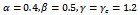
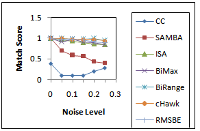
In order to evaluate implanted constant, coherent and overlap biclusters in synthetic data, we have used the technique proposed by Zimmermann et al.[9]. For constant bicluster generation, we adopt the following steps:

a. Generate a 100 × 100 matrix A with all elements 0

b. Generate ten biclusters (modules) of size 10 × 10 with all elements 1

c. Replace elements of biclusters with random noise val-ues from uniform distribution (-σ,σ)

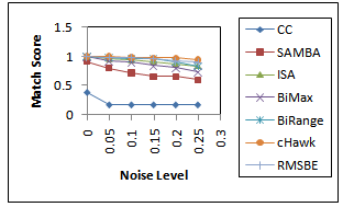
For all experimentation, we set the noise level range from 0.0 to 0.25. In case of overlapping biclusters, we used 10 degrees of overlap where the size of matrix and bicluster vary from 100 × 100 to 110 × 110 and from 10 × 10 to 20 × 20, respectively. The steps for evaluation of coherent biclusters are same as that of constant bicluster, but rows and columns in a bicluster have a 0.02 increasing trend. The parameter setting for different algorithms is shown in Table 2. In order to validate the accuracies of different algorithms, we apply the gene match score proposed by Zimmermann et al.[9]. Let and be two sets of biclusters. The match score of with respect to is given by:

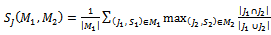(1)

where J and S are set of genes and a set of conditions in a bicluster respectively. Let represent the set of implanted biclusters and M be the set of output biclusters of an algorithm. The score represents the degree of similarity between extracted biclusters and the implanted biclusters, where as the score represents how well each of the true biclusters extracted by the bicluster algorithm.

Figure 3 illustrates the experimental results with respect to the accuracy evaluation of constant biclusters. As per the experimental results, in case of high noise level for extraction of constant biclusters; BiRange along with cHawk, ISA and RMSBE shows high accuracies; BiMax and SAMBA perform moderately, and CC perform poorly. Figure 4 illustrates the experimental results with respect to the accuracy evaluation of coherent biclusters. For coherent biclusters, BiRange has a comparable accuracy with RMSBE and cHawk. Figure 5 illustrates the experimental results with respect to the accuracy evaluation of overlapped biclusters. In case of overlapped biclusters, BiRange is marginally affected by the overlap degree of the implanted biclusters.

Table 2. Parameter Settings for Different Biclustering Techniques S. N. Algorithm Setting 1 BiRange 2 SAMBA 3 CC 4 cHawk 5 BiMax 6 RMSBE 7 ISA

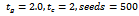
Figure 3. Accuracy of Constant Biclusters

Figure 4. Accuracy of Coherent Biclusters

Figure 5. Accuracy of Overlapped Biclusters

4.2.3. Real Dataset

For real gene expression dataset, provided by Gasch et al.[17], the performance of the proposed technique BiRange is evaluated with respect to other similar algorithms based on the methodology used by Zimmermann et al.[9]. In order to evaluate extracted biclusters for their enrichment level based on Gene Ontology (GO) annotations[21], a web tool called FuncAssociate[22] is also used. The adjusted significance scores (α) were computed using FuncAssociate and is shown in Figure 6. The experimental results for BiRange is compared with other algorithms like BiMax, RMSBE, cHawk, SAMBA, ISA and CC based on this significance score.

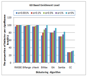Figure 6. Proportion of GO Based Enriched Biclusters

4.2.4. Performance of BiRange

In this section the performance of the proposed BiRange algorithm is analyzed. We have synthetically generated datasets with sizes ranging from 2000 × 100 to 100000 × 500 and implant constant biclusters in this matrix. Figure 7 illustrates the performance of BiRange, cHawk and RMSBE with respect to execution time for different size of dataset. As per our complexity analysis, the execution time of BiRange increases approximately linearly with the number of genes in a cluster, while execution time for RMSBE increases at a much higher rate. This confirms the practical applicability of our proposed algorithm.

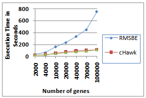Figure 7. Performance of BiRange, cHawk and RMSBE

5. Conclusions

We have represented the gene expression data using a weighted range bipartite graph, by computing the weight of each gene for a specified condition pair. For the construction of bipartite graph, the set of experimental conditions are partitioned into two disjoint sets based on the rank of valid edges. The rank value is computed from the cardinality of the corresponding gene-set, which is associated with the valid edge. The motivation of considering conditions as vertices of the bipartite graph is due to large number of genes in real gene expression data. The proposed algorithm has been evaluated for synthetic as well as real microarray data. The experimental results reveal the effectiveness of our approach over other biclustering approaches with respect to time.

ACKNOWLEDGEMENTS

We would like thank the anonymous referees for their invaluable comments and suggestions that greatly improved the quality and presentation of this paper.