1. Introduction

Major Histocompatibility Complex (MHC) molecules are cell membrane proteins which play a very important role in the immune system through the process of antigen presentation. The outer extracellular domains of these molecules form a cleft in which a peptide fragment is bound. These peptides are derived from proteins degraded inside the cell, including both self and foreign protein antigens. MHC molecules bound to peptides are carried to the cell surface where they present their cargo to T cells. This antigen presentation process is essential for the recognition of the antigen by T cell receptors. MHC molecules are of two classes: Class I and Class II. Class I is responsible for presentation of peptides of intracellular origins e.g. self-antigens and viral peptides. These Class I molecules are present on all nucleated cells and present peptides to cytotoxic T cells. Class II is responsible for presentation of peptides of extracellular origins e.g. endocytosed and digested bacterial antigens. These Class II molecules are present on specialized immune system cells called Antigen-Presenting Cells(e.g. macrophages and dendritic cells) and they present peptides to helper T cells. Naïve helper T cells when exposed to APCs with MHC Class II loaded with an antigen start to proliferate and differentiate into Effector T helper cells (Memory T helper cells and Regulatory T helper cells) with their specific roles adaptive cellular and humoral immunity. From the above we can see the importance of having the ability to determine which peptides bind to MHC-II molecules in the development of epitope-based vaccines and immunotherapeutics for infectious diseases, cancer and autoimmune diseases that are better tolerated and have fewer side effects than conventional vaccines.

MHC Class II molecules are characterized by having a peptide-binding groove that is open at both ends which allows peptides of great variability (typically 11 to 30 amino acids) in length to bind to these molecules[1]. This variability in length complicates computational approaches for the prediction of the core nonamer essential for binding. However, several studies indicate that a core of nine amino acids is the most essential part in the binding[2,3].

Several computational methods for the in silico prediction of MHC-II binding peptides have been proposed including: evolutionary algorithms and artificial neural networks[4], particle swarm optimization[5], hidden Markov models[6], Gibbs sampling[7], support vector machines[8] and ant colony search[9]. These computational methods can be used to reduce the number of candidate peptides that will be used in a wet-lab for further testing thus reducing time and cost of the development of new epitope-based vaccines.

In this study we propose a new approach, EpiGASVM, based on evolutionary algorithms and support vector machines. We have used evolutionary algorithms as a tool to search for the core binding nonamers. We then calculated the similarity scores between each pair of nonamers using BLOSUM62 substitution matrix and we used the resulting similarity matrix as input to a Support Vector Machine using Radial Basis Function (RBF) Kernel to produce the final classification results. We have tried this approach on a similarity-reduced dataset of known binders and non-binders. The dataset was originally extracted from IEDB and is composed of 12 allele datasets. From each allele dataset we selected 60 instances (30 binders and 30 non-binders). We have split the data into training and test subsets of 40 and 20 balanced instances respectively. We calculated the prediction accuracy and area under the receiver operating characteristics curve (ROC) to measure the performance of each variation of EpiGASVM.

2. Methods

2.1. Datasets and Data Preparation

In a study by El-Manzalawy et al.[10] it was demonstrated that the predictive performance of algorithms applied to the MHC Class-II prediction problem is affected by the peptide similarity in the training and test data.We have utilized similarity-reduced datasets available from the Repository of Epitope Datasets (RED)[11] to provide more accurate performance results of EpiGASVM.

The dataset was originally extracted from IEDB (identified by IEDB-SRDS2 in[10]) and we refer to it as the IEDB dataset from this point forward. In[10] the author details the methodology that was used for the similarity reduction in 3 sequential steps namely: filtering to select unique peptides followed by filtering to ensure no pair of peptides shares a 9-mer subsequence then finally filtering to ensure that the sequence identity between any 2 pairs is less than 80%.

We prepared the datasets by randomly selecting 30 unique binders and 30 unique non-binders from the RED datasets to produce a 60 instance balanced dataset for each allele (12 alleles for the IEDB data). Each of these datasets was used with the 9 variations of EpiGASVM to produce the results reported in this work.

2.2. Idea

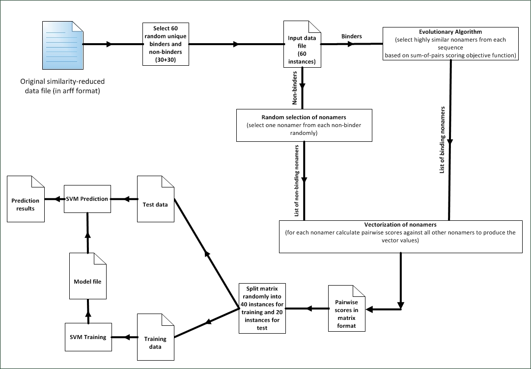
As a result of the great variability in length of MHC Class-II binding peptides and the fact that a 9-mer core is critical for binding and since typically we try to test several peptides at a time, an exhaustive search methodology would be impractical. We have utilized several variations of evolutionary algorithms to search for the core nonamer by locating the most similar nonamers in all of the sequences under test. Similarity between nonamers is calculated by using pairwise scores between each participating nonamer. The higher the score the more similar the nonamers and consequently the more probable that these selected nonamers are the core nonamers that binds in the MHC-II groove.The similarity score is calculated based on the values of the BLOSUM62 substitution matrix. Each individual that’s progressively developed in the EA is a representation of a list of nonamers and the fitness value of this individual is the sum of all pairs of similarity scores of all participating sequences. As the generations of the EA progress, the individuals of population are developed and the selected nonamers change with the hope of finding more fit individual which represents a more similar set of nonamers.

We run our variations of EA against known binders to produce a list of most similar nonamers that represent our positive instances. We then select randomly one nonamer from each non-binder to complement the dataset with negative instances. The list of positive and negative nonamers (binders and non-binders) is vectorized by calculating the pairwise similarity score for each nonamer against the rest of the nonamers in the list. The output from this step is a list of vectorized nonamers which are split into training data and test data for the support vector machine. The SVM is trained using the training data to produce a prediction model and then the prediction model is tested using the test data to calculate the final prediction accuracy. The process is illustrated in “Figure. 1”.

2.3. Evolutionary Algorithms

Evolutionary algorithms (EAs) are a group of metaheuristic optimization algorithms which are designed to optimize an objective function through providing a set of solutions (individuals) that are iteratively developed and improved over time using operators that are biologically inspired e.g. selection, recombination, mutation, etc. The iteration in an EA is usually called a generation and each generation, with the exception of the first one which is randomly generated, is developed from members of the previous generation by applying the genetic operators on members of the previous generation. This is motivated by a hope that the new population will present better solutions to the objective function.

2.4. Population Structure

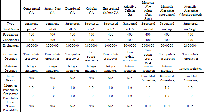
Evolutionary algorithms can be classified based on the structure of the population into: structured EAs and non-structured (panmictic) EAs. In panmictic EAs there exists a single population that includes all the individuals (solutions) under evaluation and consequently genetic operators are applied to all members of the population as a whole e.g. recombination can occur between any two members of the population. On the other hand, structured evolutionary algorithms present multiple sub-populations where genetic operators are applied within the sub- population. The structuring of the population provides some benefits like better sampling of the search space and the ability to balance the exploration/exploitation power of the algorithm.

Since the fitness landscape for our problem is unknown, we experimented with structured EAs as well as panmictic EA. Experimentation with structured EAs gave us the ability to control the trade-off between exploration and exploitation[12]. This allowed us to tailor the algorithm to thenature of the problem by giving it more explorative power to escape local maxima/minima or by giving it more exploitative power to converge quickly to a global maximum/ minimum.

We have developed nine variations of EpiGASVM that differ in the implemented EA (two panmictic algorithms: Steady-State GA and Generational GA, and seven structured algorithms: distributed GA, cellular GA, adaptive cellular GA, hierarchical cellular GA, and three memetic algorithms). We have utilized Simulated Annealing (SA) as a local search strategy in the 3 memetic algorithms which differ in the way the locality of the neighbourhood is defined as follows:

Neighbourhood: the candidate solutions are randomly selected from the same cell of the individual under consideration.

Population: the candidate solutions are randomly selected from the whole population.

Random: the candidate solutions are randomly generated by assigning arbitrary values to all genes of the individual.

More detailed information about the various EAs discussed in this section can be found in[12]. We have utilized the JCell Framework[13] for the implementation of the various evolutionary algorithms discussed in this paper. The information about the nine evolutionary algorithms used inthis paper and their configuration is summarized in Table 1.

2.5. Genetic Representation

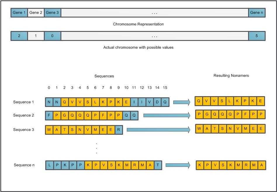
Each individual in the population is a solution to our problem; basically it is a representation of a multiple alignment of the participating sequences. A chromosome (individual) is formed of several genes and each gene is an integer representing an offset into the sequence in the range of[0, n-9] where n is the length of the sequence. This offset is used to calculate the start point of the core nonamer in the respective sequence. “Figure. 2” illustrates the genetic representation.

Figure 1. Process Overview

Table 1. Evolutionary Algorithms Summary

Figure 2. Genetic Representation

2.6. Objective Function

We utilized a sum-of-pairs objective function (1) to be maximized by the evolutionary algorithm. The scores are calculated using the BLOSUM62 substitution matrix. For each individual in the population the value of the genes are used as an offset into the sequences to obtain a list of nonamers. For each possible pair of nonamers a score is calculated and the summation of all scores is the overall fitness of individual.

The function sub() calculates the pairwise substitution scores between each residue in the nonamers S_i, S_j:

(1)

2.7. Termination Criteria

We have set the termination criteria to 400 generations or 1000,000 evaluations of the objective function for all of our evolutionary algorithms whichever is reached first with the exception of memetic algorithms which are given 2000,000 evaluations due to the local search step which adds to the number of evaluations done.

2.8. Vectorization and Normalization of Nonamer Instances

The output from the EA techniques mentioned above is a list of nonamers that are known binders. This list is combined with a list of randomly selected nonamers from known non-binders. The vectorization is done by calculating the pairwise score between each pair of nonamers in the combined list using the BLOSUM62 substitution matrix, a technique similar to the technique of Liao et al.[14]. This is followed by normalization of each vector in the range[-1,1].

2.9. Support Vector Machines

Support vector machine (SVM) is a well-established supervised learning technique that has been used extensively in many fields including bioinformatics. The SVM provides binary classification for linearly non-separable data by mapping this data to a higher dimensional space where the data is likely to be separable and then finding the hyperplane with the largest margin in this high dimensional space that can be used for differentiating positive from negative samples. The SVM classification is done in two steps: a training step where the SVM is trained on a sample of the data with known class labels to produce a classification model and test step where the constructed model is applied to the rest of the data to produce the classification result.

We have utilized SVM with the Radial Basis Function (RBF) Gaussian Kernel. The data of each allele is composed of 60 instances, 40 of which were used as training samples and 20 for test. The RBF kernel hyper parameters (C, γ) were determined by using 5-fold cross validation and grid search on all the data (60 instances)[15]. We have utilized LibSVM library for our SVM work[16].

3. Results and Discussion

3.1. Algorithm Performance

We have plotted the fitness value of the best individual against the number of generations performed by each EA for all sets of data to demonstrate the convergence speed of each algorithm. In terms of speed, the steady-state genetic algorithm has achieved the apparent optimum fitness on 4 of 12 datasets faster than the other 8 algorithms we used. This is followed in ranking by adaptive cellular genetic algorithm (achieving optimum in 3 out 12 sets faster than the other algorithms). Table 2 shows fastest converging algorithm variant for each allele.

On the other end of the scale, the memetic algorithm with the local search restricted to the neighborhood (maNeigh) shows the worst performance, failing to achieve the apparent optimum on 11 out of 12 datasets within the bounds of the stopping criteria. This is followed in ranking by generational genetic algorithm (failing 10 out 12 datasets). Table 3 shows the algorithms failing to reach the apparent optimum on each allele.

Table 2. Best Convergence Speed for each Allele Dataset Algorithm DRB1-0101 acGA DRB1-0301 ssGA DRB1-0401 ssGA DRB1-0404 cGA DRB1-0405 hcGA DRB1-0701 genGA DRB1-0802 acGA DRB1-1101 dGA DRB1-1302 ssGA DRB1-1501 ssGA DRB4-0101 dGA DRB5-0101 acGA

3.2. Prediction Accuracy and Area under ROC Curve

We have split each dataset into 40 instances used for training and 20 instances used for test and we have calculated the prediction accuracy and area under the receiver operating characteristic curve. On the IEDB dataset we have achieved an average accuracy of 90.46% and an average area under the curve of 0.9654. Table 4 lists the accuracy values and the Table 5 lists the ROC values achieved.

In terms of prediction accuracy the steady-state genetic algorithm shows the best performance on the IEDB dataset with average prediction accuracy of 93.75% but in terms of AUC the cellular genetic algorithm shows the best performance with an average AUC of 0.9808 on the same dataset.

3.3. Performance Comparison to State-of-the-Art Techniques

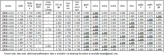
We compared our work to the techniques included in a recent study by Wang et al.[17] in which the authors compared the performance of 7 approaches for the prediction of MHC Class-II epitopes on similarity-reduced data. In their paper Wang et al. compared the performance of Average Relative Binding matrix (ARB)[18], PROPRED[19], SMM- Align[20], combinatorial library, NN-Align[21], a consensus of all previous 5 methods and a consensus of 3 methods (NN-Align, SMM-Align, Combinatorial Library or PROPRED). Table 6 shows a comparison of these methods against our 9 approaches using the AUC.

Table 3. Algorithms Failing to Reach Global Optimum Dataset Algorithm DRB1-0101 ssGA, genGA, hcGA, dGA, cGA, maPop, maNeigh DRB1-0301 genGA, acGA, hcGA, dGA, cGA, maRnd, maPop, maNeigh DRB1-0401 genGA, hcGA, dGA, maNeigh DRB1-0404 ssGA, genGA, hcGA, dGA, maPop, maNeigh DRB1-0405 ssGA, genGA, acGA, dGA, cGA, maRnd, maPop, maNeigh DRB1-0701 ssGA DRB1-0802 ssGA, genGA, hcGA, dGA, maRnd, maPop, maNeigh DRB1-1101 ssGA, genGA, acGA, hcGA, cGA, maRnd, maPop, maNeigh DRB1-1302 dGA, maPop, maNeigh DRB1-1501 genGA, acGA, dGA, cGA, maRnd, maNeigh DRB4-0101 ssGA, genGA, maPop, maNeigh DRB5-0101 ssGA, genGA, hcGA, dGA, cGA, maRnd, maPop, maNeigh

Table 4. Prediction Accuracy Family genGA ssGA acGA hcGA dGA cGA maRnd maPop maNeigh Min Max Avg DRB1-0101 85.00 90.00 80.00 80.00 75.00 85.00 80.00 85.00 85.00 75.00 90.00 82.78 DRB1-0301 95.00 100.00 95.00 90.00 85.00 90.00 95.00 90.00 95.00 85.00 100.00 92.78 DRB1-0401 80.00 90.00 85.00 90.00 85.00 90.00 90.00 90.00 90.00 80.00 90.00 87.78 DRB1-0404 90.00 85.00 90.00 90.00 85.00 100.00 95.00 90.00 85.00 85.00 100.00 90.00 DRB1-0405 95.00 100.00 85.00 95.00 85.00 100.00 85.00 90.00 90.00 85.00 100.00 91.67 DRB1-0701 90.00 100.00 85.00 90.00 90.00 95.00 95.00 95.00 95.00 85.00 100.00 92.78 DRB1-0802 90.00 100.00 90.00 90.00 95.00 95.00 85.00 90.00 90.00 85.00 100.00 91.67 DRB1-1101 100.00 95.00 90.00 75.00 100.00 80.00 95.00 95.00 85.00 75.00 100.00 90.56 DRB1-1302 95.00 85.00 85.00 95.00 95.00 95.00 100.00 100.00 85.00 85.00 100.00 91.67 DRB1-1501 95.00 100.00 85.00 90.00 95.00 95.00 85.00 90.00 90.00 85.00 100.00 91.67 DRB4-0101 100.00 85.00 95.00 95.00 90.00 85.00 90.00 95.00 90.00 85.00 100.00 91.67 DRB5-0101 95.00 95.00 90.00 85.00 95.00 95.00 85.00 80.00 95.00 80.00 95.00 90.56 Min 80.00 85.00 80.00 75.00 75.00 80.00 80.00 80.00 85.00 75.00 85.00 80.00 Max 100.00 100.00 95.00 95.00 100.00 100.00 100.00 89.58 95.00 95.00 100.00 97.78 Avg 92.50 93.75 87.92 88.75 89.58 92.50 90.00 89.58 89.58 87.92 93.75 90.46

Table 5. Area under ROC Allele genGA ssGA acGA hcGA dGA cGA maRnd maPop maNeigh Min Max Avg DRB1-0101 0.9800 1.0000 0.9300 0.9100 0.8800 0.9200 0.9600 0.9100 0.9600 0.8800 1.0000 0.9389 DRB1-0301 1.0000 1.0000 0.9700 0.9700 0.9700 0.9900 0.9900 0.9700 1.0000 0.9700 1.0000 0.9844 DRB1-0401 0.8900 0.8900 0.9300 0.9600 0.9600 0.9800 0.9900 1.0000 0.9900 0.8900 1.0000 0.9544 DRB1-0404 0.9500 0.9400 0.9500 0.9000 0.9400 1.0000 0.9800 0.9600 0.9400 0.9000 1.0000 0.9511 DRB1-0405 0.9700 1.0000 0.9700 0.9500 0.9200 1.0000 0.9200 0.9000 0.9300 0.9000 1.0000 0.9511 DRB1-0701 0.9000 1.0000 0.9100 0.9900 0.9500 0.9900 0.9800 1.0000 0.9900 0.9000 1.0000 0.9678 DRB1-0802 1.0000 1.0000 1.0000 0.9100 0.9900 0.9800 1.0000 0.9900 0.9600 0.9100 1.0000 0.9811 DRB1-1101 1.0000 0.9400 0.9700 0.8700 1.0000 0.9400 1.0000 1.0000 0.9600 0.8700 1.0000 0.9644 DRB1-1302 0.9800 0.9900 0.9600 0.9900 0.9300 1.0000 1.0000 0.8500 0.9800 0.8500 1.0000 0.9644 DRB1-1501 1.0000 1.0000 0.9900 0.9600 1.0000 1.0000 0.9500 1.0000 0.9200 0.9200 1.0000 0.9800 DRB4-0101 1.0000 0.9200 1.0000 1.0000 0.9500 0.9700 0.9800 0.9500 0.9900 0.9200 1.0000 0.9733 DRB5-0101 1.0000 1.0000 1.0000 0.9800 0.9700 1.0000 0.9900 0.8200 1.0000 0.8200 1.0000 0.9733 Min 0.8900 0.8900 0.9100 0.8700 0.8800 0.9200 0.9200 0.8200 0.9200 0.8200 0.9200 0.8911 Max 1.0000 1.0000 1.0000 1.0000 1.0000 1.0000 1.0000 1.0000 1.0000 1.0000 1.0000 1.0000 Avg 0.9725 0.9733 0.9650 0.9492 0.9550 0.9808 0.9783 0.9458 0.9683 0.9458 0.9808 0.9654

Table 6. Comparative AUC data for ARB, PROPRED, Combinatorial Libraries, SMM-Align, NN-Align, Consensus, Consensus3 and the variations of EpiGASVM

4. Conclusions

We have developed a new technique, EpiGASVM, for the MHC-II epitope prediction problem. The prediction accuracy and AUC achieved on 12 similarity-reduced datasets shows that EpiGASVM is reliable and accurate. According to our knowledge, the accuracy and AUC achieved with EpiGASVM is the best in the field for the MHC-II prediction problem and it’s our hope that this new technique will be an addition to the arsenal of tools available for researches for the rational design of new epitope based vaccines and immunotherapeutics.