-
Paper Information
- Paper Submission
-
Journal Information
- About This Journal
- Editorial Board
- Current Issue
- Archive
- Author Guidelines
- Contact Us
International Journal of Astronomy
p-ISSN: 2169-8848 e-ISSN: 2169-8856
2023; 12(1): 1-11
doi:10.5923/j.astronomy.20231201.01
Received: Feb. 19, 2023; Accepted: Mar. 4, 2023; Published: Mar. 21, 2023

Nutation and Chandler Wobble in a Model of the Rotating and Undulating Curved Surface of Space-time in the Solar System
 Abstract
 Reference
 Full-Text PDF
 Full-text HTML
Adrián G. Cornejo
Electronics and Communications Engineering from Universidad Iberoamericana, Santa Rosa 719, CP 76138, Querétaro, Mexico
Correspondence to: Adrián G. Cornejo, Electronics and Communications Engineering from Universidad Iberoamericana, Santa Rosa 719, CP 76138, Querétaro, Mexico.
| Email: |  |
Copyright © 2023 The Author(s). Published by Scientific & Academic Publishing.
This work is licensed under the Creative Commons Attribution International License (CC BY).
http://creativecommons.org/licenses/by/4.0/

Based on the Schwarzschild metric, the Flamm’s paraboloid of revolution, and the Lense–Thirring precession, we explore a model in which the entire Solar System rotates and undulates the curved surface of space-time that forms it. This model considers the representation of a curved space-time surface as an undulated four-dimensional surface in rotation with vertex at the Sun. With this model, the rate of apsidal precession, axial precession, nutation and Chandler wobble of the Earth can be predicted from a rotating and undulating Solar System scenario. In this approximation, nutation and Chandler wobble can be described as arbitrary oscillations in the Earth’s orbit as it traverses an undulating space-time surface while orbits. According to this model, planets and other celestial bodies in the Solar System would oscillate when orbiting around the Sun, forming the rate of the observed nutation and Chandler wobble of the Earth and Mars while the system is in rotation. The undulations on the curved space-time surface would resemble consecutive waves as in a fluid in rotation. The curved space-time geometry of the Solar System can be observed from pictures taken from orbiting spacecraft. Then, we estimate in this model the orientation of the Earth’s North Pole with respect to curved space-time, considering that the North Pole must point towards the inner Solar System.
Keywords: Schwarzschild metric, Flamm’s paraboloid, Lense–Thirring precession, Nutation, Chandler wobble
Cite this paper: Adrián G. Cornejo, Nutation and Chandler Wobble in a Model of the Rotating and Undulating Curved Surface of Space-time in the Solar System, International Journal of Astronomy, Vol. 12 No. 1, 2023, pp. 1-11. doi: 10.5923/j.astronomy.20231201.01.
Article Outline
1. Introduction
- The entire Solar System is considered to remain static while the planets orbit around the Sun. However, what effects would there be if the entire Solar System rotates and undulates the curved surface of space-time that forms it? And would such effects match some of the known observations? In General Relativity [1], the Einstein field equations describe the metric of the four-dimensional space-time static surface expressed by the stress-energy tensor. The concise form of the Einstein field equation is defined as
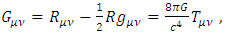 | (1) |
 | (2) |
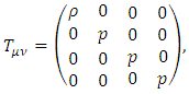
 | Figure 1. Three-dimensional representation of the geometry of the Einstein’s equation that describes the universe as a spherical surface (for simplicity) supporting enough matter-energy at the point P to curve the spherical surface. RU is the radius of the universe |
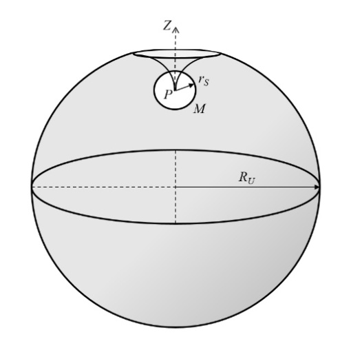
 | Figure 2. Three-dimensional representation of three possible forms of curvature of space-time static surface, according to General Relativity: (a) The so-called “flat” universe in the Einstein equations for vacuum, when Rμν = 0. (b) Enough matter and energy to curve space-time static surface, as in the case of moons and planets, among other celestial bodies. (c) Curvature of the space-time static surface due to a star or a black-hole singularity at a point P |
1.1. Elliptical Orbits in the Schwarzschild Metric
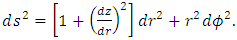
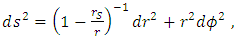
- An exact solution of the Einstein field equations was developed by Schwarzschild [2], which describes a four-dimensional curved space-time static surface in the vacuum for a static (non-rotating) and spherically symmetric star or black-hole singularity. The Schwarzschild metric resembles a Flamm’s paraboloid of revolution about the Z-axis [3] (similar to a “curved cone”) which does not include the Schwarzschild radius. It can be derived as follows. The Euclidean metric in the cylindrical coordinates (r, φ, z) is written as
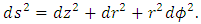 | (3) |
 | (4) |
 | (5) |
 | (6) |
 | (7) |
 | (8) |
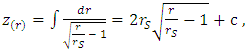
 we can write this equation as the static surface of a paraboloid (with vertex at the origin) in the form
 | (9) |
 | (10) |
 | (11) |
 | (12) |
 | (13) |
 | (14) |
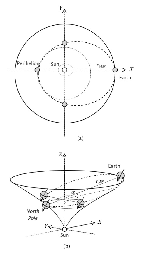 | Figure 3. (a) Top view representation of the Earth’s orbit on the XY-plane, in a planar geometry of the Solar System. (b) Three-dimensional representation of the lateral view of the considered curved geometry of space-time static surface of the Solar System with vertex at the Sun, and with the Earth’s orbit on the tangent plane to the curvature, according to the Schwarzschild metric |
1.2. Tilt of the Orbital Plane and the Ecliptic in the Schwarzschild Metric
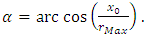
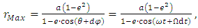
- In the Flamm’s paraboloid, the tilt of an orbital plane with respect to the XZ-plane is the tangent to the curve at the furthest point of the orbit with respect to the focus. In the Solar System, the distance rMax = a(1 + e) is the maximum Planet-Sun distance during aphelion, where a is the semi-major axis of the ellipse and e its eccentricity.A right triangle can be formed in the XZ-plane with the maximum distance (rMax) as hypotenuse (see Figure 4), given as
 | (15) |
 | (16) |
 | (17) |
 | (18) |
 | (19) |
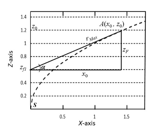 | Figure 4. In a curved space-time static surface representation, a right triangle is formed with the maximum distance to the Sun (rMax) as the hypotenuse. The tilt angle 𝛼 is the tilt of the orbital plane tangent to the curvature in the XZ-plane |
 | (20) |
|
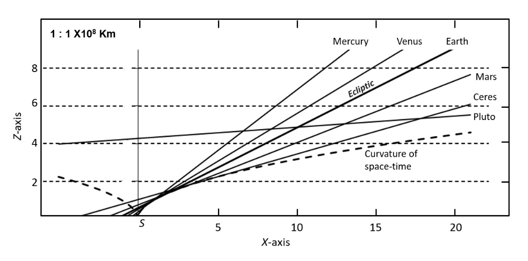 | Figure 5. Representation of the tilt of the orbital planes of some celestial bodies as tangents to the four-dimensional curvature of the static surface in the Flamm’s paraboloid (dashed line). The Sun (S) at the origin |
1.3. Apsidal Precession of the Elliptical Orbits in the Schwarzschild Metric
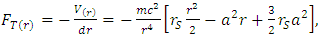
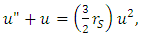
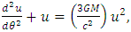
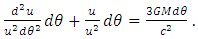
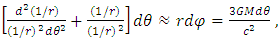
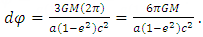
- One of the first predictions of the GTR was the correct calculation to determine the advance of Mercury’s perihelion [6]. Since then, this calculation has been developed by different methods, giving the same result. According to the Schwarzschild’s metric, the effective potential can be written as
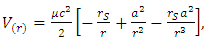 | (21) |
 | (22) |
 | (23) |
 | (24) |
 | (25) |
 | (26) |
 | (27) |
 | (28) |
 | (29) |
1.4. Apsidal Precession from the Lense-Thirring Dragging Effect Revisited
- Some works [7,8] consider, in a Friedmann–Lemaître (FL) geometry, that both the curvature of space-time surface described by General Relativity and the accelerated expansion of the universe [9,10] considered from the Hubble observations, provide both the dynamics and the curved geometry of space-time surface in the presence of a massive body. However, outside the expansion dynamics of the universe, these possible forms of curved space-time surface are considered static (i.e. no rotational dynamics is considered) around stationary mass distributions. In addition, some works [11-15] consider the scenario in which the entire Solar System would be rotating around a spin axis at the Sun and with a specific angular velocity.Regarding rotating systems, the gravitation of a spinning spherical massive body of constant density was studied by Lense and Thirring [16]. We can consider the Lense–Thirring precession, which is a relativistic correction to the precession of a rotating body, such as a gyroscope, near a large rotating mass, such as the Earth or the Sun (which has a mass of approximately 1.99 × 1030 kg, and rotational velocity of approximately 1,997 km‧s-1) [17]. This effect is due to the rotation of the central mass. It is a prediction of General Relativity consisting of secular precessions of the longitude of the ascending node and the argument of pericentre of a test particle freely orbiting a central spinning mass endowed with angular momentum S. The metric is given as
 | (30) |
 | (31) |
 | (32) |
 | (33) |
 | (34) |
 | (35) |
 | (36) |
 | (37) |
 | (38) |
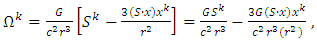 | (39) |
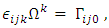
 is the ordinary flat-metric inner product of the position and the angular momentum. That is, when the gyroscope’s angular momentum relative to the fixed stars is Li, then it precesses as
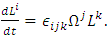 | (40) |
 | (41) |
 | (42) |
 | (43) |
 | (44) |
 | (45) |
 | (46) |
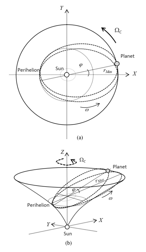 | Figure 6. Three-dimensional representation of the apsidal precession (like the precession of Mercury’s perihelion) in a four-dimensional rotating reference frame. (a) Top view representation. (b) Lateral view representation |
 | (47) |
1.5. Axial Precession in the Rotating Reference Frame
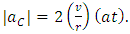
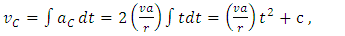
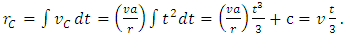
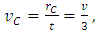
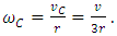
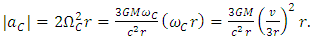
- Considering a model of the rotating Solar System, such a kind of rotation should be perceived from Earth as a change in linear position with respect to the observed “fixed” stars, noting that these would have an apparent periodic circular motion. Indeed, this effect is the observed in axial precession. From Eq. (44) and considering the angular velocity in terms of Coriolis acceleration, yields
 | (48) |
 | (49) |
 | (50) |
 | (51) |
 | (52) |
 | (53) |
 | (54) |
 | (55) |
 | (56) |
 | (57) |
 | (58) |
 | (59) |
 | (60) |
 | (61) |
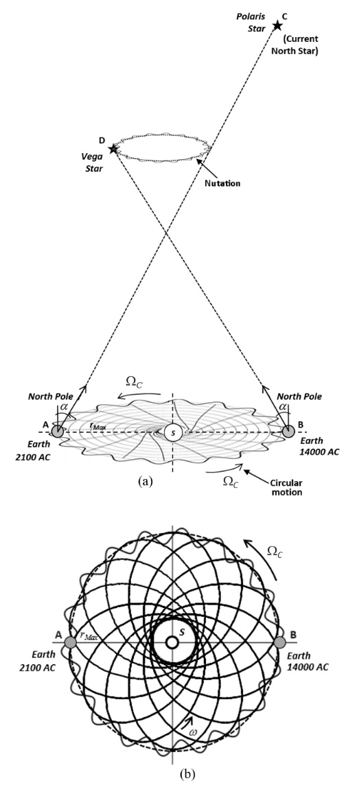 | Figure 7. (a) Three-dimensional representation of the path of the Earth orbiting and rotating in a rotating system with undulations to form the observed nutation with respect to the “fixed” stars. (b) Top view representation of the rosette-like path of the Earth orbiting and rotating in a rotating system with undulations to form the observed nutation with respect to the “fixed” stars |
2. Model of Nutation as Undulations Along the Space-Time Surface in the Rotating Reference Frame
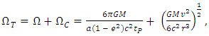
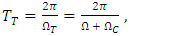
- Nutation is considered a slight irregular movement in the axis of rotation of symmetrical objects that rotate on their axis [19]. In the case of the Earth, the nutation is superimposed on the axial precession motion and the swaying of the obliquity of the ecliptic so that they are not regular, but rather wavy. The nutation of the Earth causes that every 18.6 years the axis of rotation of the Earth apparently oscillates up to about 284.28 m (9.2 seconds of arc) on each side of the mean value of the obliquity of the ecliptic. It is considered that the other planets also produce variations, called perturbations, but these are of a small value to be considered to affect these planetary movements. Since nutation is an additional axial motion superimposed to the axial precession, in this model nutation is considered as the oscillation of the orbit due to the undulations of the space-time surface that a planet follows while orbits. Therefore, we can model the geometry of curved space-time surface in rotation accordingly to the observed nutation. In this model, Earth (as well as the other planets) follow the undulated shape of the rotating curved space-time surface with crests and troughs along the orbital path. To comply with the observed nutation, we arbitrarily add a term which builds the oscillations to the rotating curved space-time surface [20], in order to model and resemble the nutation movement. From Eq. (58), this model can be written as
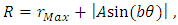 | (62) |
3. Model of Chandler Wobble as Undulations Along the Rotating Curved Space-Time Surface
- The Chandler wobble or Chandler variation of latitude is a small deviation detected in the Earth’s axis of rotation [21]. The Chandler wobble is superimposed on the nutation and on the axial precession motion. It is considered as a nutation. It amounts to change of about 9 m at the point at which the axis intersects the Earth’s surface and has a period of 433 days [22]. In the same way, we arbitrarily add a second term which builds the oscillations of the rotating curved space-time surface, in order to model and resemble the Chandler variation. Considering Eqs. (58) and (60), the equation that describes the spinning of the curved space-time surface with crests and troughs along this movement, is modelled as
 | (63) |
3.1. Spiral Behavior in the Dynamics of a Rotating Reference Frame
- As also considered in a previous work [15], from Eq. (22) and in the same way as with the equation for classical mechanics scenario to define the orbital velocity, we equate the centrifugal force with the given third term which consider the correction from General Relativity, obtaining
 | (64) |
 | (65) |
 | (66) |
 | (67) |
 | (68) |
 | (69) |
 | (70) |
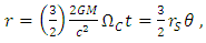
 | Figure 8. (a) Top view representation of the rotating and undulated curved space-time surface in the Solar System. (b) Three-dimensional representation of the lateral view of the considered rotating and undulated curved geometry of space-time surface in the Solar System, resembling a rotating vortex with crests and troughs and with the vertex at the Sun, and with the Earth’s orbit on the tangent plane to the curvature |
3.2. Chandler Wobble of Mars in the Rotating Reference Frame
- With radio tracking observations of the Mars Reconnaissance Orbiter, Mars Odyssey and the Mars Global Surveyor spacecraft, the Chandler wobble of Mars was detected. The detected amplitude is 10 cm, the period is 206.9 ± 0.5 days and it is in a nearly circular counterclockwise direction as viewed from the North Pole [24]. Modelling the shape of the rotating space-time surface, adding the Chandler wobble of Mars, it can be consistent with nutation and Chandler wobble in Earth and Mars, as
 | (71) |
 | (72) |
4. The Position of the Earth in the Curved Space-time Surface in the Solar System
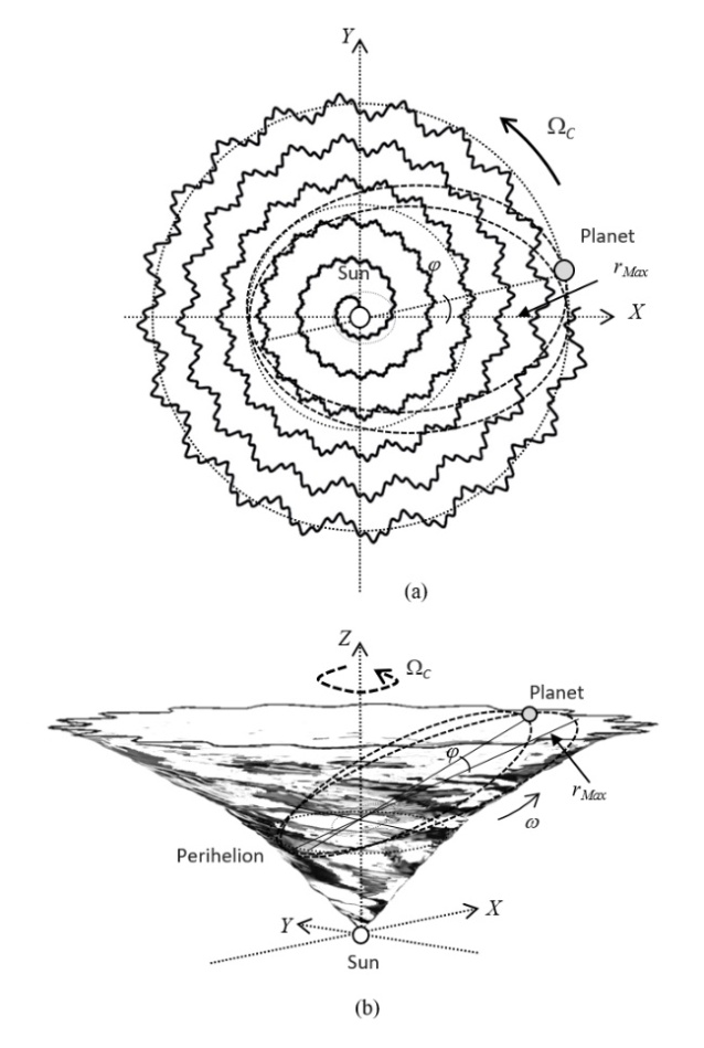
- Considering the image of Earth (moving away from its perihelion) and Jupiter (moving away from its aphelion) during an alignment with Mars, taken on May 8th, 2003 from the Mars Global Surveyor (NASA) orbiting spacecraft pictures [26,27] to graphically determine the direction in which the North Pole of the Earth points with respect to the Solar System.From this picture and considering that the orbit of Mars is between the orbits of Earth and Jupiter, we note that the Earth’s South Pole is fully visible and pointing towards Jupiter, which appears in the image at a great “vertical” distance d from the Earth. This means that the Earth’s South Pole must be pointing towards the outer Solar System, while the North Pole must be pointing towards the inner Solar System (see Figure 9). The direction of the Earth’s North Pole is also shown in Figure 3(b). Thus, having Jupiter below in the picture and the Earth above (closer to the Sun), the Sun must be positioned at the top of the picture.
 | Figure 9. Representation of the isometric projection of the geometry of curved space-time surface in the Solar System from an interpretation of the Mars Global Surveyor picture (May 8, 2003) |
5. Conclusions
- The aim of this work is to explore a model of a rotating and undulating curved space-time surface in the Solar System from a post-Newtonian scenario. In this way, the consideration of the rotational and undulation dynamics of the Solar System allows to consider the curved space-time surface to comply with some known movements of the Earth, such as the apsidal precession, axial precession, nutation and Chandler wobble from this scenario. Then, the geometry and rotational dynamics of curved space-time surface in the Solar System is modelled with undulations, in which the orbits can match with the nutation and Chandler wobble, resembling an undulating surface as a rotating vortex in spiral with vertex in the Sun. In this way, the apsidal precession, the axial precession, nutation and Chandler wobble of the Earth and Mars can be modelled from the Flamm’s paraboloid as undulated and in rotational dynamics. From satellite pictures and observations, the position and geometric orientation of the Earth with respect to curved space-time surface can be estimated, considering that the North Pole must point towards the inner Solar System. The next step in proving the dynamics of rotation and undulation of the curved space-time in the Solar System is to make more precise and detailed observations of its angular momentum and relative motion with respect to other celestial bodies, in order to confirm if the way in which space-time rotates and undulates in the Solar System agrees with these considerations and can be predicted by the dynamics described in this model.
ACKNOWLEDGEMENTS
- The author would like to thank Professor Sergio S. Cornejo for its review and comments for this work.
Appendix A. The Rosette-Like Path of a Body Orbiting and Rotating Around a Fixed Axis
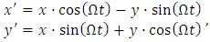
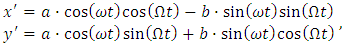
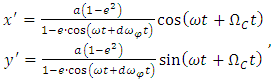
- The elliptical path of a body periodically orbiting around a fixed axis in a static circular reference frame as described by the Kepler’s laws shows a simple harmonic oscillator with angular frequency ω. Elliptical path in parametric equations, is given as
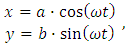 | (73) |
 | (74) |
 | (75) |
 | (76) |
 | (77) |