1. Introduction

There is now considerable evidence that the motion of the different celestial bodies is not random [1, 2]. In particular, research has found that celestial bodies are attuned to gravitational resonances involving the Fibonacci numbers [2]. Current practice has been to use a ratio unit as the basis for comparing celestial resonance periods. Yet, the sinusoidal component parameters of celestial bodies may also refer to a certain time unit of the Fibonacci numbers. Such a time unit approach may provide a new method to investigate the hierarchical stability of the solar system. Thus, in this study, a time-unit approach was used to investigate the correlation of Fibonacci numbers and celestial mechanical cycles including the period of rotation, precession, and orbit. The Fibonacci series was measured in 24-hour and 365-day units of time. It was hypothesized that celestial mechanical cycles would be associated with the Fibonacci numbers expressed in 24 hours because of the unique self-organizing properties enabled by 24-hour periodicity.

2. Method

2.1. Data Analysis

Data were collected on known celestial mechanical cycles. The cycles included rotation period, precession period, and the orbital period. Correspondence between celestial mechanical cycles and Fibonacci numbers was assessed by subtracting the celestial cycle value from the Fibonacci number to obtain a deviation percentage. Fibonacci numbers were chosen for comparison on the basis that they were the closest in proximity to the celestial mechanical cycle. The differences in the average deviation values were analyzed for commensurability. Conventionally, a 5% rejection region is taken to indicate statistical significance [3]. Thus, in the analysis, this was used as the cut-off for significance. That is, if a data set falls within 5% of the actual value of the Fibonacci series on either side (plus or minus), the data is close enough to the actual value that it can be treated as statistically significant. On the other hand, if the average deviation is outside this limit, then such differences can be accounted for by random error.

2.2. Measurements and Calculations

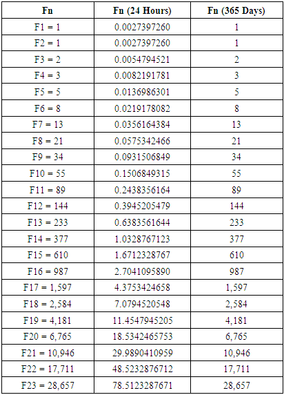
The Fibonacci series may essentially be expressed in two units of time: the 24-hour daily rotation of the earth and 365-day orbit around the sun (see Table 1). In the first method of measurement (Table 1, Column 2), each Fibonacci number is divided by 365, since in one day, the Earth travels about 1/365 of the way around the sun. For example, the first Fibonacci number (Column 2, Row 2) expressed in a 24 hour unit of time is approximately 1/365. This produces a constant accrual rate with the interesting properties of the Lucas numbers and the powers of Phi. The Lucas numbers are in the following integer sequence: 2, 1, 3, 4, 7, 11, 18, 29, 47, 76, 123, etc. The Lucas numbers use the same recurrence relation as the Fibonacci numbers but with initial values 2 and 1 instead of 0 and 1. Similarly, the powers of Phi approach the values of the Lucas numbers: Phi¹ = 1.6180, Phi² = 2.6180, Phi³ = 4.2361, Phi⁴ = 6.8541, Phi⁵ = 11.0902, Phi⁶ = 17.9443, Phi⁷ = 29.0345, Phi⁸ = 46.9787, Phi⁹ = 76.0132, etc.

Table 1. The Value of Each Fibonacci Number Given in Two Units of Measurement

In the second method of measurement (Table 1, Column 3), each Fibonacci number can be expressed in a 365 day unit of time. In comparing the two methods, the time scaling will influence the absolute magnitudes of time parameters, but not how they are distributed (the ratios will remain the same). Thus, the differences are based on absolute time parameters rather than proportional distributions.

3. Results

3.1. Rotation Period

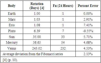
The rotational period of a celestial object is the time taken for it to complete one rotation around its own axis relative to the background stars. The analysis examined the rotation period for the Sun, Planets, and Dwarf Planets. Only rotation periods greater than one day were examined. Statistical analysis was not able to be performed with the Fibonacci numbers expressed in 365 days for lack of sufficient whole number comparison. A table detailing the correspondences between the rotation period and the key study variables is shown in Table 2 (Note: adding all Fibonacci numbers expressed in 24-hours produces a pattern of numbers—1, 2, 4, 7, 12, 20—that are each one number off from the Fibonacci numbers). In line with predictions, the average deviation was statistically related to Fibonacci numbers expressed in 24 hours (2.13%). Thus, Fibonacci numbers expressed in a 24 hour unit of time successfully predicted rotation period.

Table 2. Rotation Period for the Sun, Planets, and Dwarf Planets

3.2. Precession Period

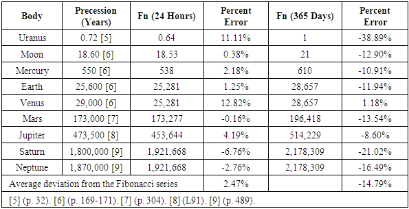
Next, it was tested whether Fibonacci time cycles predicted precession of the planets and moon. Precession is the slow change in the orientation of a planet due to gravitational torques exerted by other solar system bodies in which the tip of the axis rotates (precesses) just as a spinning top does. The Sun also has precession, but it is exceedingly small because of the Sun’s nearly spherical shape, fast rotation rate, and limited gravitational torque from other bodies. A table detailing the correspondences between precession and the key study variables is shown in Table 3. In line with predictions, the average deviation was statistically related to Fibonacci numbers expressed in 24 hours (2.47%), and not statistically related to Fibonacci numbers expressed in 365 days (-14.79%). Thus, Fibonacci numbers expressed in a 24 hour unit of time successfully predicted precession.

Table 3. Precession Period for the Planets and Moon

3.3. Orbital Period

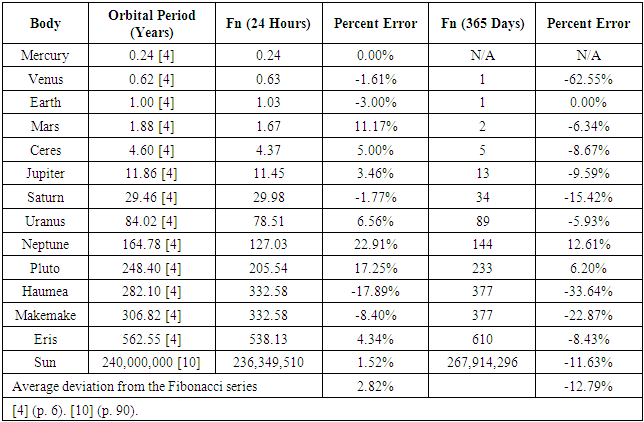
Finally, it was tested whether Fibonacci time cycles predicted orbital periods of the Sun, Planets, and Dwarf Planets. The orbital period is the time a given astronomical object takes to complete one orbit around another object. It applies to planets orbiting the Sun, and the Sun orbiting the galaxy. A table detailing the correspondences between the orbital period and the key study variables is shown in Table 4. In line with predictions, the average deviation was statistically related to Fibonacci numbers expressed in 24 hours (2.82%), and not statistically related to Fibonacci numbers expressed in 365 days (-12.79). Thus, Fibonacci numbers expressed in a 24 hour unit of time successfully predicted the orbital period.

Table 4. Orbital Period for the Sun, Planets, and Dwarf Planets

4. Discussion

The present results show that the Fibonacci resonances in celestial mechanics are more than ratio-based. The Fibonacci series expressed in 24 hour-based units was associated with several celestial cycles. Specifically, the Fibonacci series expressed in 24 hour-based units predicted the period of rotation, precession, and orbit across multiple time scales. Perhaps as important, it was found that the Fibonacci series in year-based units did not predict celestial mechanics. It seems that a critical consequence of the Fibonacci series is that it entrains celestial dynamics based on a 24-hour periodicity and not a 365-day periodicity. This, in turn, contributes to the stability of the solar system.

This data provides an explanation for why rotation and orbital resonances are linked to ratios in accordance with the Fibonacci series [2]. That is, the harmonic ratios observed are explained by hierarchical entrainment of oscillations in keeping with the Fibonacci series expressed in a 24 hour unit of time. Mathematically, it could be argued that the significance of the number 24 may be due, at least in part, to the 24 repeating digits of the Fibonacci series [11]. Not only do the 24 repeating digits of the Fibonacci series themselves approximate a sine wave [11], but just as a sine wave has alternating positive and negative phases, so too the Fibonacci series has alternating positive and negative phases. This is further evidence suggesting that the Fibonacci series corresponds to a sine wave.

The alternating positive and negative phases of the Fibonacci series are indicated by taking the ratio of every adjacent number in the series (see Table 5). Table 5 shows how the ratios of the successive numbers in the Fibonacci series quickly converge on the golden ratio (0.618…). Notice that as we continue down the sequence there is an alternating bigger (+) and smaller (-) pattern. For example, the ratio 2 divided by 3 is 0.666 (+), and 3 divided by 5 is 0.60 (-). The basic Fibonacci sine wave pattern has implications that might extend to quantum mechanics and the observable properties of a system. To draw such a conclusion or indication for quantum mechanics, it may be noted that the golden ratio and Fibonacci numbers appear in quantum mechanics [12-14].

Table 5. The Alternating Positive and Negative Phases of the Fibonacci Series

Matter has the property of “self-organization.” The term self-organization refers to emergent order in complex systems. Self-organizing systems create spontaneous order from local interactions between the parts of the system. The process of self-organization can be found in many fields ranging from plasma physics [15]; chemistry [16], psychology [11], cybernetics [17], and biology [18]. In planetary physics, the principle of self-organization has been applied to harmonic orbit resonances [19], Jupiter’s or Saturn’s rings and moons [20], protoplanetary disks [21-22], and Jupiter’s Red Spot [23]. In astrophysics, self-organization has been applied to galaxy and star formation [24], magnetic reconnection [25]; planetary atmosphere physics [23]; magnetospheric physics [26], ionospheric physics [27], solar magnetic fields [28]; and solar corona physics [29].

Self-organization in the solar system is related to gravitational resonances [19-20, 30]. The simplest case of a gravitational resonance happens when the orbital periods of two planets have an integer ratio relationship (e.g., 1:2, 3:5, etc.). More complex gravitational resonances occur when one considers the planetary precession periods in addition to their orbital periods. Strong and weak resonances pervade the solar system. The present results help to understand how overlapping resonances (i.e., multiple gravitational resonances in close proximity) achieve global stability of the whole planetary system. Each planet contributes gravitational influence to the system such that the resulting tidal forces provide a positively or negatively reinforcing effect upon the celestial objects of the system. Orbital periods and cyclical motions of any kind may be represented as sine waves possessing frequency and amplitude. When perturbations are in phase with the motion of a celestial object, the amplitude of the cyclical motion increases. Similarly, perturbations that are out of phase decrease the amplitude of the cyclical motion. Thus, the resonant structure in a gravitationally interacting oscillating system could be explained by the action of gravitational perturbations [30].

Just as a composite waveform may be decomposed into a set or spectrum of individual waves, the gravitational resonances of the solar system can be represented as a sum of oscillating waves to produce a single composite waveform [19]. This mode of representation is known as harmonic analysis or spectral analysis. The statistical technique of spectral analysis is used to discover cyclic components in a time series [31]. Spectral analysis averages times series and presents the information as a function of wavelength. Waves are analogous to numbers in this regard. Each wave is analogous to a number that may be added or subtracted from the others to create a final number, denoting a “constant function.” This process of summing harmonic modes of a fundamental wave may be used to mathematically re-construct any waveform or constant function by applying the rules of constructive and destructive interference. Regarding solar system stability, gravitational resonance is analogous to a constant function resulting from the summation of interacting oscillating periods around the mean of the Fibonacci series expressed in 24-hour units of time.

The orbits of planets in our solar system self-organized and evolved over the eons into highly regular gravitational resonances. Though not all planets in the solar system possess highly regular gravitational resonances, our solar system continues to evolve into a state of increasing stability as time progresses [30]. On the macrocosmic scale, the complex gravitational resonances of the solar system arise from entrainment to the Fibonacci series expressed in 24-hour units of time. Moreover, the Fibonacci series describes the spiral geometry of many galaxies. On the microcosmic scale, the golden ratio and Fibonacci numbers also appear in atomic physics and quantum phase transition [12–14]. Matter exists in the Universe because elementary particles are products of a natural harmonic order based on the golden ratio (as well as its rational form, the Fibonacci sequence). The structural composition of atoms is not arbitrary; symmetry and uniformity exist at every level of scale. Consistent and straightforward mathematical rules of symmetry always apply, giving rise to a dynamic fractal unifying interaction based on the golden ratio.

5. Conclusions

Gravitation is thought to be responsible for the cohesion of our planetary system and a critical organizing principle of matter. Gravitational resonance implies that specific harmonic configurations are repeated. According to the present findings the Fibonacci series expressed in a unit period of 24 hours, and not a unit period of 365 days, was significantly correlated to celestial mechanical cycles. These considerations hold for the period of rotation, precession, and orbit. Thus the conclusion is that the hierarchical stability of the solar system is related to the Fibonacci series expressed in a unit period of 24 hours. Ultimately, these results can help to provide a deeper theoretical understanding of the mechanisms of resonance and long-term stability in the solar system.