I. A. Atoum, M. Ali
Department of Computer Science and Software Engineering, College of Computer Science and Engineering, University of Ha’il, Ha’il, Kingdom of Saudi Arabia
Correspondence to: I. A. Atoum, Department of Computer Science and Software Engineering, College of Computer Science and Engineering, University of Ha’il, Ha’il, Kingdom of Saudi Arabia.
| Email: |  |
Copyright © 2012 Scientific & Academic Publishing. All Rights Reserved.
Abstract
Solar filaments are large regions of very dense, relatively cool ionized gases when compared with the surface of the sun, held in place by magnetic fields. These filaments usually appear above the chromosphere as thin elongated structures. The filaments are usually associated with the occurrence of coronal mass ejections (CMEs). CMEs are major solar eruptions that may cause geomagnetic storms on Earth. Thus, a more efficient filament detection algorithm, being a development of the work of Qahwaji and Colak back in 2005 is presented in this paper for extracting the spine of solar filaments. A geometrical-based approach is used for extracting the filament spine and determining its properties. The accurate detection of the filament’s spine could provide an accurate description for the shape, size and orientation of the filament. The method introduced in this work is fullyautomated and near real-time while the previous works depend on using a priori constant values.
Keywords:
Solar image, Solar filament, Filament detection, Automatic detection, Spine, Coronal Mass Ejection (CME)
Cite this paper: I. A. Atoum, M. Ali, Automated Algorithms for Detecting Solar Filaments in H-Alpha Solar Images and Detecting Their Spines, International Journal of Astronomy, Vol. 2 No. 4, 2013, pp. 56-64. doi: 10.5923/j.astronomy.20130204.02.
1. Introduction
Detecting and characterizing solar filaments is important for different aspects of solar activities because of their association with geomagnetic storms, as presented in[1]. In this paper, we present an automated computer system that processes full-disk Hα solar images to detect filaments, extract their boundary and spine. This method includes three major stages; firstly, the detection algorithm is able to detect solar filaments from region-grown images. Secondly, the filament boundary is determined using morphological operations. Finally, the spine description algorithm has the ability to represent the spine as a smooth curve, which passes through the middle of the boundary data. Solar filament detection is a challenging process because solar filament appearance and shape could change across different images. In addition, efficient detection systems should be fully automated and work in real-time, which makes their development harder. In this paper, we will tackle some of these challenges.There were some successful attempts for designing algorithms for detecting solar features. In[2] a detection method based on thresholding and region-based growing techniques were introduced. A technique that depends on thresholding and morphological filtering was used to isolate filaments from Hα images in[3]. In[4] they have used a feed-forward neural network for detecting solar filaments in the Hα images, The technique utilizes two hidden neurons and one output neuron to distinguish between the background and the filament. In[5] the detection process uses an algorithm that belongs to a family of partial differential equations to enhance solar filaments. Then support vector machine (SVM) was used to differentiate between the sunspots and filaments. In[6] a region growing technique was used to segment the filament areas; followed by applying an iterative thinning method to produce the skeleton of the region; thereafter a pruning process is used to remove the branches of the skeleton tree.A different new method is implemented by[7] that use an intensity and size threshold to extract filaments. In terms of accuracy and similarity of the algorithms, our algorithm was compared with this work. A fast, novel, accurate and robust automated algorithm is presented in this paper, which is capable of detecting solar filaments and describing its spine. The detection method is unlike its predecessors, it has avoided using any empirical values to produce a fully automated techniqueThis paper extends the pioneering work in[7] to produce a fully automated filament detection algorithm that is both faster and more accurate. Definitely, the time-consuming factor will affect synthesizing a filament detecting and tracking system to be part of a proposed real-time system. Therefore, this limitation will prevent the system from producing timely space weather alerts and quick look-up results. Significantly, the accuracy of detecting the filament’s spine plays an important rôle in identifying the main attributes of the filament under consideration and as well as in achieving the subsequent processing tasks with more accuracy. Additionally, our algorithm is a geometrical-based approach, which is different from the morphological-based technique of[6], while in[7] they have used a principle curve approach. From analysis of[7], it would appear that his algorithm is the foundation of our algorithm but we have greatly extended his research in terms of speed and accuracy. This paper is organized as follows: the data used is discussed in Section Two. The automated detection technique is presented in Section Three. Section Four describes the new technique for extracting the filament’s spine. Results and evaluation are presented in Section Five, and conclusions are presented in Section Seven.
2. Data
The data used for this study are full-disk solar images (spectroheliograms) which were observed at Meudon observatory http://bass2000.obspm.fr/home.php in GIF format. The Spectroheliograph is an instrument intended to produce monochromatic images of the Sun in various wavelengths. The Meudon spectroheliograms are composed of Hα images, Ca II K1 images, Ca II K3 images, and Ca II K3 images. The Hα line is a strong spectral line (high absorption) which has a wavelength of 656.3 nm (red light). At this line we can see up to 1700 km above the visible layer as described in[8]. The spectroheliograms in which filaments are best seen are in Hα images, hence they used in this study. They provide us with a look into the chromosphere that exists above the visible photosphere of the sun and it could be observed by using the Hα line The Hα images show different solar features, plages, short-lived solar flares, sunspots, and elongated filaments. Filaments appear as dark ribbons against their brighter background.
3. Filament Detection and Boundary Extraction
In this section, the algorithms used for detecting the shape and size of the solar filaments and extracting their boundaries are described.
3.1. Background
It is important to point out that in this work the solar filament candidate detection is carried out based on the previous work of[9]. In[9], a detection process for recognizing and verifying solar filaments and active regions from Hα images was introduced. The techniques introduced in[9] is for pre-processing (cleaning and enhancement), detecting the solar disk and then applying an intensity filtering technique to detect the candidate pixels for the filaments. The process ends by applying a region growing technique to detect regions of interest that were not detected by intensity filtering alone. The use of these algorithms automatically identifies the number of filaments in each solar image, the dimension of each filament is then determined and this is shown by enclosing each filament by a rectangle. It is worth mentioning that, for the purpose of this work, the intensity filtering stage in[9] is improved by applying an adaptive thresholding technique in[10].We will follow up this method by developing a fully automated detection technique that includes retrieving the actual filament area from a region grown one.
3.2. Filament Detection
Some image artifacts exist within the h-alpha images (e.g. elliptic shapes of the solar disk, dark lines across the images, etc.), which do indeed need to be taken into account by image cleaning.[6] addressed this already. However, Fuller’s method depended mainly on using local windows of size 1/6 of the global image size and a local threshold for each of these sub-windows were then computed using a local quiet Sun intensity minus a constant value multiplied by the standard deviation. Hence, the local variations in the image, affects the accuracy of Fuller’s detection algorithm. However, our approach is different, as we have used adaptive global thresholding technique; this means our algorithm is less dependent on the local variations in the image intensity values. Taking this approach helps us to deal with both the intra-image intensity variations and across the different day images over the month being considered.To retrieve the actual filament size and shape from the region grown one that was produced by the technique of[9], a local threshold is adopted that uses the mean of the minimum and maximum values and the standard deviation. The first function: the mean of the minimum and maximum values were calculated at every pixel in the image over a sliding window of 5×5 pixel neighbourhood centred on this pixel of the region grown image. The second function: the standard deviation was calculated for the whole region grown filament. The size of the sliding window, which is 5×5 pixels, was chosen such that it would both include the smaller filaments and also exhibit a relatively more uniform image intensity variation - therefore the selected window area will not be affected much by the local illumination gradient. Using such a small window size also has the additional advantage of a fast computational time, making our algorithm perform in real-time. Then the following thresholding, given in Equation (1) is applied: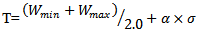 | (1) |
Where  represents the minimum value of the intensity values in the sliding windows and
  stands for the maximum value of the intensity values of the sliding window.
  stands for the standard deviation of the whole filament area. The value of α is calculated using Equation (2) for solar images from the Meudon observatory or using Equation (3) for solar images from BBSO and KANZ solar images.
 | (2) |
 | (3) |
represents the standard deviation of the intensity values in the previous sliding window. The thresholding rule is applied afterwards, which is shown in Equation (4), below: | (4) |
 represents the detected filament,
  is the region grown filament. The integer “1” is used to denote specifically the filament pixels and the integer “0” specifically for the background pixels. The mean stands for the mean value of the area of region grown filament and T is the threshold value resulting from Equation (1). Figure 1 illustrates the main steps of the filament detection technique. The result of the whole detection process is shown in Figure 2.d. Note that 2.a is the original image, 2.b is the output of the adaptive thresholding technique and 2.c is the region-grown image. This technique has the advantage of being fully automated.The output image of this detection method still suffers from existing small, unwanted pixels and small holes. These pixels needs to be removed without distorting the image, noting that it is impossible to remove such noise totally without distorting the image. Nevertheless it is a vital step in reducing the overall image noise to an acceptable level. Using morphological operators are one way that could be used to remove these pixels and fill the small holes at the same time whilst relatively preserving the corner details.
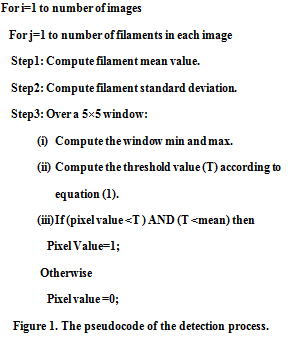 | Figure 1. The pseudocode of the detection process |
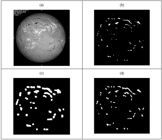 | Figure 2. The result of the whole detection process by using Hα image observed at Meudon observatory on 8th February, 2001. (a) Original Image. (b) Segmented Image. (c) Region Grown Image. (d) Detection Results |
These operators could achieve the previous task by using the combination of dilation and erosion operators. Note that they have a disadvantage in merging the close elements. However. by using a small structuring element, due to the existing small size of these spots and holes, will consequently avoid such shortcomings.The opening morphological operation has been applied using a 3×3 square structuring element to eliminate noise (small unwanted pixels in the detected image) while preserving the shape and size of the larger objects. The opening operation consists of the erosion operator followed by dilation. To remove other unwanted isolated spurious pixels, a thresholding operation has been set as given in Equation (5). If the object area is less than this threshold value, it will then be removed. Another closing operation was implemented afterwards using a 3×3 square structuring element to fill in the empty pixels left after the previous operations. The closing operation includes a dilation followed by an erosion operation. | (5) |
Where  is the mean value of the whole image,
  and
and  are the maximum and minimum intensity values of the whole image respectively. This equation was found empirically to give the best results in suppressing unwanted isolated spurious pixels.
3.3. Boundary Extraction
Determining the filament’s boundary is a necessity for subsequent activities; such as spine extraction. The final filament region was extracted after following the stages as shown in Figure 3. Additionally, in[6], they have described the spine extraction process as three different phases without any details about boundary extraction. These are the: thinning method, producing the skeleton and pruning. Morphological image processing describes a collection of image processing techniques that deal with the structure of features in an image as discussed in[11]. There are three primary morphological techniques: erosion, dilation and hit-or-miss. One application of the erosion operation is in boundary finding. The boundary is extracted by subtracting the eroded image from the original image, as shown in Equation (6), below: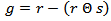 | (6) |
Where r is the image of the region under consideration, s is the structuring element (SE), Θ is the erosion operation, and g is the image of the regions boundaries. The size of the SE is chosen to be 3×3 pixels in order to identify the one-pixel-wide boundary. Figure 4.a shows a detected filament of a horizontally stretched filament, Figure 4.b shows its boundary.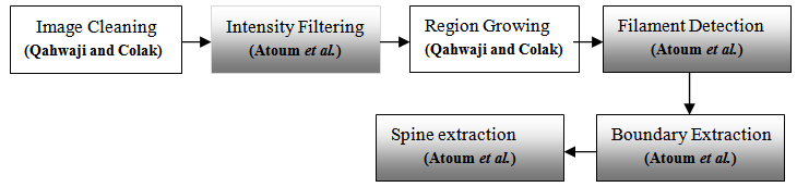 | Figure 3. The sequence of phases implemented and constructed to detect the filament disappearances. (Author’s contribution shown in shaded boxes) |
 | Figure 4. Boundary detection results by using one filament stretched horizontally of an Hα image observed at Meudon observatory on January 2, 2001. (a) Detected Filament. (b) Filament Boundary |
4. Spine Description and Extraction
The accurate detection of the filament spine could provide an accurate description of its: shape, size and orientation. An accurate spine detection algorithm should satisfy the following requirements that are mentioned in[6] and[12]:1. Non-linear summary: the spine should pass through the middle of its region, following the body of the filament as a curve not as a line.2. Morphology: the spine should retain the shape of the original feature shape.3. Adaptation: the shape of the spine should match any changes in the filament shape.4. Connectivity: The spine points should be connected.For this work, we will not be describing the spine as a set of line segments, where a threshold can be used to control their size and number as in[7]. Additionally, it does not make extensive use of the morphological operations (standard thinning and skeletonization) to extract the filament spine as done by[6], because this could require significant computational time. Instead, we propose a new automated technique for detecting and extracting these spines. This new technique has the ability to represent the spine as a smooth curve, which passes through the middle of the boundary data. This would produce a curve consisting of a set of connected points instead of line segments. To determine these curves, six consecutive steps are implemented, as shown below: The first seed pixel is determined by moving up from lower left to the lower right pixels of the rectangle that encloses the filament. When a white pixel is found, then a three line segment is drawn towards the filament body as shown in 5.b. 5.a represents a detected filament. Finally, the middle point of the longest line segment is chosen to be the seed pixel for drawing the spine, as shown in Figure 5.c. Moving to the next vertex requires drawing the full line segments that passes through the seed pixel (the first vertex determined above in Figure 5.c) towards the boundary of the feature as shown in Figure 5.d and then choosing the largest line segment as shown in Figure 5.e, this segment will guide the spine for the opposite longest line segment as shown in Figure 5.f; which will determine the starting point of the spine and will complete the drawing of the full spine. The final phase of the algorithm is the most important. For each point in the largest line segment, we find the mid-point of the perpendicular line segments that intersects this line; i.e. if the first drawn line is horizontal then the projection will be achieved by finding all the mid-points of the vertical lines that intersect this line as shown in Figures 6.a and 6.b.
 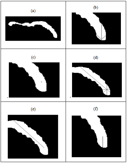 | Figure 5. The steps implemented for spine determination. (a) Solar filament. (b) The three line segments. (c) The middle of the longest line segment. (d) The full four line segments that pass through the seed pixel. (e) The longest line segment. (f) The opposite longest one of e |
Finally, to prevent repeating the drawing of the four line segment step, the previous drawing direction is preserved as a reference for the next movement. This requires ignoring any direction that will guide the spine to go back to its previous starting position as shown in Figure 6.d.The resulting discrete curve is represented as discontinuous points, some of these points were missed because finding the mid-point of the perpendicular line segments that intersects the largest line segment produces a consecutive discrete points as shown in 7.a, which at the end needs to be connected. So, an algebra slope-intercept algorithm described by[13] is used to connect these separated points by drawing lines between them as shown in Figure 7.b. In this algorithm any straight line on the coordinate plane can be described by the equation ax+by+1=0.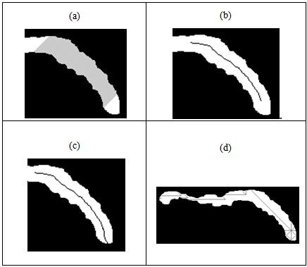 | Figure 6. Projecting and averaging phase of determining the spine. (a) The projection result. (b) The averaging result. (c) The first longest line segment and its opposite longest one. (d) The continuity while preserving the previous orientation to determine the next movement |
 | Figure 7. The result of applying the slope-intercept algorithm. (a) Before applying the algorithm. (b) After applying the algorithm |
The final curve is shown in Figure 8, below: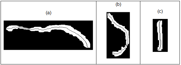 | Figure 8. The Full Filament Spine: (a) Full spine of a horizontally stretched filament. (b) Full spine of a filament from an Hα image observed at BBSO observatory on 9th February, 2002. (c) Full spine of a vertically stretched filament |
5. Results
In order to demonstrate the performance of our algorithm, the results were compared with Bernasconi et al. (2005). The two algorithms were applied to one hundred different-sized filaments collected empirically from different images, which are: 1/1/1999, 2/1/1999, 3/1/1999, 2/1/2001, 3/1/2001, 4/1/2001, 29/7/2 001, 30/7/2001 and 31/7/2001. It was clear that the filament spine in Bernasconi et al. (2005) is more suitable for large filaments. Thus, using a spine length of 20 pixels chosen by Bernasconi et al. (2005), was the most appropriate for them, as they were using larger filaments to process. It is also apparent that our algorithmically derived spine is more convoluted, precisely because it accurately follows the body of the filament - as it goes through the middle of the feature as shown in Figure 9.b. Figure 9.a shows the original filament. Determining the first guess line as explained in Bernasconi et al. (2005) by running roughly parallel to the longest side of the box that tightly encloses the filament under consideration. Figure 9.d shows the output if the first guess line is chosen as in Figure 9.c where  is the longest side of the box (one of the longest sides of the box that encloses the filament), while Figure 9.f shows the drawn spine if the first guess line is chosen as in Figure 9.e where
  is the longest side of the box that encloses the filament. If the first guess line is chosen as in Figure 9.g, the line produced by going from c to d row-by-row going up until we get on end-point, the output will be as shown in Figure 9.h. These results illustrate the better accuracy of our algorithm, which is a characteristic of crucial importance for the automatic determination of the filament spine.
5.1. Efficiency of the Algorithm
The algorithm introduced here is computationally less complex compared to[7]. The former on average takes 0.098 s to extract the filament spine, while the latter takes 0.341 s. The computer used in this work is an Intel Core Duo CPU P8700, 2.53 GHz, running the Windows Vista 32-bit operating system. Figure 10 shows the processing times for the whole sample composed of one hundred features.Additionally, our implementation results in a longer spine length because it tracks the actual filament backbone more accurately as shown in Figure 9. This result in a longer spine length and this is indeed confirmed by the longer pixel count of our spines as shown in Figure 11, compared against[7]’s results. 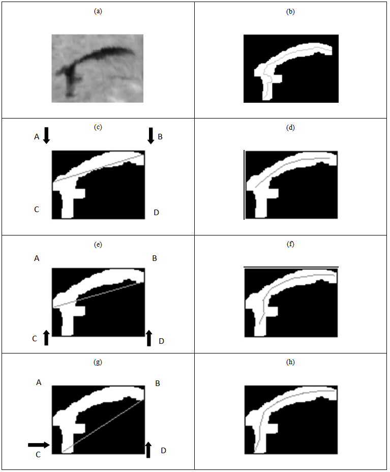 | Figure 9. Samples illustrating the filament tortuousness and accuracy of the spines from Atoum (b) and Bernasconi (d, f, h) algorithms. (a) Original filament. (b) Spine produced using Atoum algorithm. (c) The first guess Line  . (d) The spine produced using the (c) guessed line. (e) The first guess line . (d) The spine produced using the (c) guessed line. (e) The first guess line  . (f) The spine produced using the (e) guessed line. (g) The first guest line produced by row and column processing (h) The spine produced using the (g) guessed line . (f) The spine produced using the (e) guessed line. (g) The first guest line produced by row and column processing (h) The spine produced using the (g) guessed line |
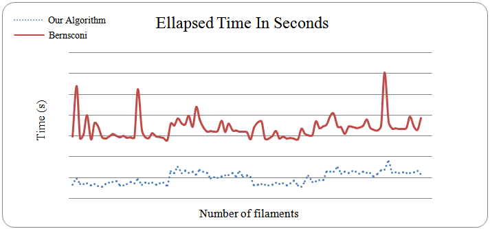 | Figure 10. Elapsed Time in seconds per feature for the two algorithms |
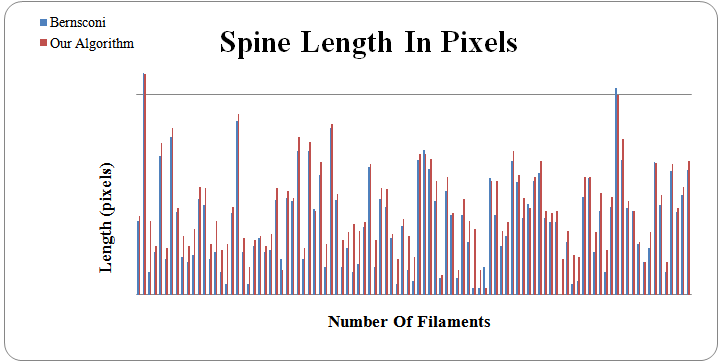 | Figure 11. Spine length in pixels per feature |
6. Conclusions
A novel algorithm has been developed and presented in this paper for fully automating the detection of solar filaments by manipulating statistical parameters and morphological operations. Our detection process is fully automatic and does not use any empirical values. The shape of the detected features are represented by determining its spine geometry. The algorithm gives the opportunity to extract all the filament morphological features, such as: filament length, filament center, filament head end-points, filament tail end-points and filament boundary. The algorithm is valuable as part of a real-time system for detecting and tracking solar filaments. The comparison with other researchers shows that our algorithm represents the filaments more accurately and is it is also evaluated computationally faster, which could lead to a more precise tracking practice in real-time. There are, however, some problems still to be resolved. There are still cases of incomplete spines existing due to choosing the largest line segment in a wrong direction, which at the end produce imperfect drawn spine.In the future, we plan to improve and extend our algorithm to develop a filament merging technique that will join the filament broken structures, if they exist, and tracking techniques which will be able to track the day-by-day evolution for each selected filament on the Sun’s surface. This tracking of the filament disappearance is important as it affects the Earth’s space weather system. Additionally, the system will be tested with more images, with the aim of producing a new filament catalogue.
ACKNOWLEDGEMENTS
The authors wish to thank the Meudon observatory in France, and the Big Bear Solar Observatory in California (BBSO) for providing the Hα full-disk solar images for this study.
References
| [1] | Al-Omari M., Qahwaji R., Colak T. and Ipson S. S., 2010, Machine Learning-based Investigation of the Associations between CMEs and Filaments. Solar Phys. 262 (2), 511-539. DOI: 10.1007/s11207-010-9516-5. |
| [2] | Gao, J., Wang, H. and Zhou, M., 2002, Development of an Automatic Filament Disappearance Detection System, Solar Phys. 205 (1), 93-103. |
| [3] | Shih, F. Y., and Kowalski, A. J., 2003, Automatic Extraction of Filaments in H-alpha Solar Images, Solar Phys. 218 (1-2), 99-122. |
| [4] | Zharkova, V. V., and Schetinin, V.,2005, Filament Recognition In Solar Images With The Neural Network Technique. Solar Phys, 228(1-2), 137-148. |
| [5] | Qu, M., Shih, F. Y., Jing, J., and Wang, H., 2005, Automatic Solar Filament Detection Using Image Processing Techniques, Solar Phys. 228 (1-2), 119-135. |
| [6] | Fuller, N., Aboudarham, J., and Bentley, R. D., 2005, Filament Recognition and Image Cleaning on Meudon Hα Spectroheliograms. Solar Phys. 227 (1), 61-73. |
| [7] | Bernasconi, P. N., Rust, D. M., and Hakim, D., 2005, Advanced Automated Solar Filament Detection and Characterization Code: Description, Performance and Results. Solar Phys. 228 (1-2), 97-119. |
| [8] | National Solar Observatory (1996). Ca K and H Alpha Images Explained.[ONLINE] Available at:http://eo.nso.edu/MrSunspot/answerbook/cak_ha_expl.html.[Last Accessed 9 April 2012]. |
| [9] | Qahwaji, R., and Colak, T., 2005, Automatic Detection and Verification of Solar Features, Int.J.Imaging Systems Tech. 15 (4), 199-210. |
| [10] | Atoum, I .A., Qahwaji, R. S., Colak, T., and Ahmed, Z. H., 2009, Adaptive Thresholding Technique for Solar Filament Segmentation. Ubiquitous Computing and Communication Journal. 4 (4), 91-95. |
| [11] | Efford, N., 2000, Digital Image Processing, A Practical Introduction Using Java, 1st edn. Pearson Education Limited, Addison Wesley, USA. |
| [12] | Ingrid Y., Koh, Y., Lindquist, W.B., Zito, K., Nimchinsky, E. A., and Svoboda, K.: 2002, An Image Analysis Algorithm for Dendritic Spines. Neural Computation. 14 (6), 1283–1310. |
| [13] | Hearn, D., and Baker, M.P., 1997, Computer Graphics C Version. 2nd edn, Prentice Hall, Inc., New Jersey, USA. ISBN 0-13-530924-7. |
 Abstract
 Reference
 Full-Text PDF
 Full-text HTML