Philipp Kornreich
EECS Department, Syracuse University Syracuse, N. Y. 13244, US
Correspondence to: Philipp Kornreich, EECS Department, Syracuse University Syracuse, N. Y. 13244, US.
| Email: |  |
Copyright © 2012 Scientific & Academic Publishing. All Rights Reserved.
Abstract
An information based model is used to reanalyze the Cosmic Background Radiation (CBR) measured by the Cosmic Background Explorer, COBE, NASA satellite. The advantages of this mathematical model are that a radiation scattering parameter and the temperature at the detector can be calculated. from the data. Three models, the simple Black Body Radiation (BBR) curve, a model by D. J. Fixsen1 et al. and the Information Based Model (IBM) where compared to the measured data. The best X2 fit was obtained for the IBM. For the monopole radiation one obtains a temperature of 2.72503 oK and a scattering parameter of zero. For the dipole radiation a temperature of 3.285843 oK and a scattering parameter r equal to 2.0705567 is obtained.
Keywords:
Cosmic Background Radiation, Information Theory, Scattering
Cite this paper:
Philipp Kornreich, "Information Model of Cosmic Background Radiation", International Journal of Astronomy, Vol. 1 No. 5, 2012, pp. 114-120. doi: 10.5923/j.astronomy.20120105.06.
1. Introduction
In a previous paper1 the properties of the Cosmic Background Radiation (CBR) were analyzed using a Black Body Radiation (BBR) model and a BBR model that included a chemical potential. Also the author of this paper thanks D. J. Fixsen1 et. al. for the excellent processing of the measured data.Here an Information Based Model (IBM) is used to reanalyze all the data. The analysis includes the effect of scattering of the radiation. The same model is used both for the monopole and dipole data discussed by D. J. Fixsen at al1. This model does not require the postulating of an additional chemical potential. All parameters are derived from basic principles, though the exact form of one of the functions had to be assumed. The model reverts to the standard BBR theory in the limit of no scattering. The data was obtained by the Far Infra Red Absolute Spectrometer FIRAS on board the Cosmic Background Explorer COBE NASA satellite. Three models, the simple BBR curve, a model by D. J. Fixsen et al. and the IBM where compared to the measured data. The best X2 fit was obtained for the IBM.The IBM, describes radiation that traveled through a scattering medium from a hot body. Using this model the temperature and a scattering parameter can be calculated. The conventional BBR function used in the analysis of thermal systems is derived by the use of Statistical Mechanics. The model used here is derived using Information Theory.The basis of Information Theory was developed by C. E. Shannon2 at Bell Laboratories. The information theoretical model facilitates the inclusion of the effect of information propagating through noisy channels. This provides for including the effect of the thermal radiation being scattered on the way from the hot Black Body source to the detector.The energy of the electromagnetic radiation oscillating with any given frequency is divided into energy quanta or photons. The information transmitted at any frequency by the hot body is encoded in the number of photons radiated. Different number of photons radiated represent different information, see Fig. 1. The amount of information in each photon packet is not equal to the number of photons but to a function of the number of photons. This is illustrated in Fig 1. The photon packets are represented by mail bags in Fig. 1. The information in each mail bag is displayed on the tags. The units of information used in this schematic representation is in binary bits. However, the information used in this article is in Joules per Kelvin.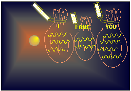 | Figure 1. Schematic representation of information transmitted by a hot object. The information is encoded in the number of photons transmitted. The amount of information in each photon packet is a function of the number of photons in the packet. The photon packets are represented by mail bags here. The information in each mail bag is displayed on its tag |
The photons travel through space where some are absorbed or scattered. Maybe, the radiation when passing trough a charged cloud is even amplified by stimulated emission. This can occur by generating additional photons of the same frequency as the incoming radiation and neutralizes some of the charges.One result of including the effect of scattering is a blue shift of the distribution of photons, see Fig. 2. Unlike in the case of the Doppler effect the wavelength of the individual photons does not change. However, the distribution changes to more short wave photons. The total number of photons can, also, change to fewer or more photons.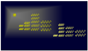 | Figure 2. Schematic representation of a blue shifted photon distribution. Unlike in the case of the Doppler effect the wavelength of the individual photons does not change. However, the distribution changes to more short wave photons |
2. Information Model
The IBM for thermal radiation through a scattering medium is analyzed below. The concepts used here can be found in a paper by C. E. Shannon2 and many Probability texts3,4,5. The information is encoded by the number n of photons radiated by the hot object, see Fig. 1. The value of each of the information packets hn is a function of the number n of photons. The information packets are shown schematically as mail bags in Fig. 1. | (1.1) |
where k is Boltzmann’s constant and Pn is the probability that a signal of n photons is being received. The average detected Shannon information is equal to the average value H of all the information packets.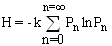 | (1.2) |
The propagation of the photons from the hot Black Body source to the detector is modeled by conditional probabilities P(m photons radiated | n Photons received) that m photons are radiated provided n photons were received. Associated with the conditional probabilities having the same condition of n photons being received are conditional entropies H(S | n). Here S is the set of all the different numbers m of radiated photons.Since the details of the scattering model are not known the conditional probabilities can not be specified. However, one can postulate a simple model for the conditional entropies4 H(S | n):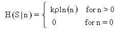 | (1.3) |
Here  is an average scattering parameter and k is Botzmann’s constant. The information I is equal to the difference between the received Shannon information H of equation 1.2 and the noise N.
 | (1.4) |
The Noise is equal to the average value of the conditional entropies H(S | n): | (1.5) |
The temperature T of the radiation at the receiver is known. | (1.6) |
where the average energy U of the received photons is given by: | (1.7) |
Its value, at this point, is not known. Here  is Plank’s constant divided by
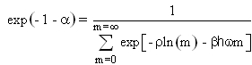
  is the oscillating frequency of the radiation.The probabilities Pn are normalized.
 | (1.8) |
The probabilities Pn can be derived by finding an extremum value of the information I subject to what is known about the system. In this case the temperature T at the receiver and the fact that the probabilities are normalized are known about the system. However, the equation 1.6 for the temperature, is not in the form of a constraint equation like equations 1.7 and 1.8. Therefore, it can not be used in this process directly. One has to use the average energy U instead, at first. By multiplying the two constraint equations, equations 1.7 and 1.8 by convenient constants  and adding them to the equation for the information I one obtains:
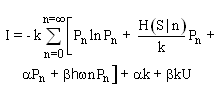 | (1.9) |
The information I will have an extremum value when all its derivatives with respect to the probabilities Pn are equal to zero. By taking the derivative of the information I with respect to one of the probabilities Pn, setting the result equal to zero and solving for the probability Pn one obtains: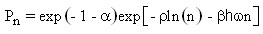 | (1.10) |
where the explicit form of the conditional entropy H(S | n) from equation 1.3 was used in equation 1.10. The values of the constants  are not known at this point. In order to evaluate the constant
  one substitutes the probability of equation 1.10 into the first constraint equation, equation 1.8 to obtain for
 | (1.11) |
The constant  can be eliminated by substituting equation 1.11 into equation 1.10.
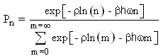 | (1.12) |
The constant  has yet to be evaluated. In order to accomplish this one, first, calculates the information of receiving n photons by taking the logarithm of the probability Pn and multiplying the result by minus the Boltzmann’s constant.
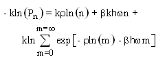 | (1.13) |
By substituting the information associate with receiving n photons, equation 1.13, into the average Shannon information of equation 1.2 one obtains: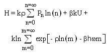 | (1.14) |
where equation 1.7 was used for the average energy U. By solving equation 1.14 for the average energy U, substituting the resulting expression into equation 1.6 and solving for  one attains the well known expression:
 | (1.15) |
The probability Pn of receiving n photons can now be completely specified by substituting equation 1.15 for the constant  in to equation 1.12
 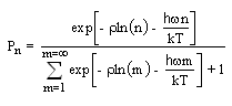 | (1.16) |
The average energy of a one dimensional radiating system where the radiation passes through a scattering medium with average scattering parameter  is derived by substituting the probability of equation 1.16 into the equation for the average received energy U, equation 1.7.
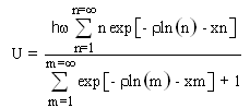 | (1.17) |
where the normalized frequency x is given by: | (1.18) |
Finally, by multiplying equation 1.17 by an appropriate density of states constant one obtains for the change  of the average received energy density u with radiation frequency
  of a three dimensional system radiating through a scattering medium:
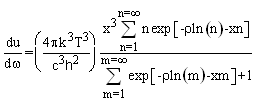 | (1.19) |
where c is the speed of light in free space. This is the Black Body Radiation law for systems radiating through a scattering medium. Note that the temperature T is the observed temperature at the receiver. Since the scattering parameter  is an Entropy amplitude it must always be positive. This shifts the peak of the distribution to larger values of the normalized frequency
  .For the case when the scattering parameter
  is equal to zero equation 1.19 reverts to the standard Black Body Radiation law.
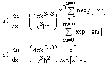 | (1.20) |
For completeness the input information I is calculated by subtracting the noise N from the Shannon information H of equation 1.4. The noise N is calculated by substituting equation 1.3 into equation 1.5. 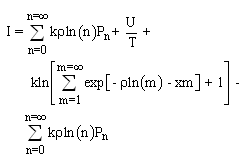 | (1.21) |
Note that the first and last terms of equation 1.21 cancel. By making use of equation 1.17 for the average energy U one obtains: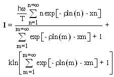 | (1.22) |
By multiplying equation 1.22 by the same density of states as was used in equations 1.18 and 1.19 one obtains: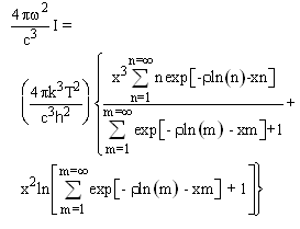 | (1.23) |
As will be shown in chapter III, RESULTS, for the CBR that the data obtained from a monopole detector exactly matches a standard BBR curve as given by equation 1.20b. However, the data from a dipole detector better fits equation 1.19. The explanation given here of the shift of the photon distribution to higher frequencies is doe to the effect of the scattering process as discussed above. This is a much simpler explanation than the one given by D. J. Fixsen et al. Thus, by Occam’s Razor, perhaps the scattering explanation is the correct one?
3. Results
a) Analysis methodIn order to determining the values of the temperature T at the receiver and the average scattering parameter  for the radiation of the CBR the data listed in Tables 1 or 2 is compared to data calculated from equation 1.19. To accomplish this comparison the observed CBR data is normalized by dividing the second column of the data by its maximum value. The data calculated from equation 1.19 is similarly normalized by dividing it by its maximum value. Next the Xi squared X2 value is calculated as follows:
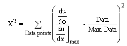 | (2.1) |
Here the normalized frequency x is.  | (2.2) |
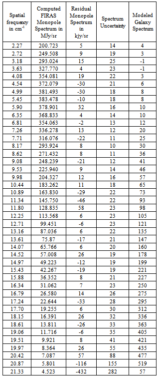
b) Analysis of monopole dataThe monopole data was measured using the FIRAS which measures the difference between the free sky radiation and an internal ideal BBR source. The data underwent substantial processing to eliminate various instrument errors. Depending on the error eliminating technique D. J. Fixsen at al1. calculate a CBR temperature of between  .The data in Table 1 was copied from “on line” NASA COBE/FIRAS Monopole data. Column 1 is the spatial frequency in units of cm-1. Column 2 is the FIRAS monopole spectrum computed as the sum of a 2.725 oK BBR spectrum and the residual in column 3. The units are MJy/sr (Mega Jansky per sterradian). Column 3 is the residual monopole spectrum from Table 4 of Fixsen et al1 in units of kJy/sr. Column 4 is the one standard deviation spectrum uncertainty from Table 4 of Fixes et al, in units of kJy/sr, and column 5 is the modeled Galaxy spectrum at the Galactic poles from Table 4 of Fixsen et al, also in units of kJy/sr.By matching the data in columns 1 and 2 of Table 1 to equation 1.19 one obtains a best fit for a temperature of 2.725(030813) oK, and a scattering parameter
  of zero for a X2 value of 1.50643015 x 10⁻⁶. This agrees well with the values calculated by D. J. Fixsen et al. Since this result was calculated from the data in Table 1 it was subject to the same error correction method used by D. J. Fixsen et al. It assumes that since the scattering parameter is an Entropy amplitude it must be positive
Table 1. Cobe/firas monopole spectrum
 |
| |
|
c) Analysis of dipole dataTable 2. (From Table 3 of D. J. Fixsen et. al.) Dipole Spectrum and Residual (Intensities in kJy/sr)
 |
| |
|
The best fit of the CBR dipole data listed in columns 1 and 2 of Table 2 to a standard BBR curve, equation 2.20b is for a temperature of 3.45306053 oK, corresponding to a X2 value of 0.10854900837.The best fit of the Cosmic Background Radiation dipole data listed in columns 1 and 2 of Table 2 to equation 1.19 occurs at a temperature of 3.285843 oK and a scattering parameter  equal to 2.0705567, see Fig. 3. at a X2 value of 0.00932734686. Thus the IBM, equation 1.19, is a much better fit to the data than the simple BBR curve. The effect of the scattering is a blue shift, see equation 1.19 and Fig. 2. of the photon number distribution observed at the receiver.Fixsen et al. used a BBR curve modified by a dimensionless chemical potential
  given by the following equation:
 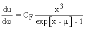 | (2.3) |
where Fixsen gives a value for the temperature T of 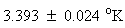 and chemical potential µ of
 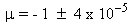 . Here CF is a density of states constant. Equation 2.3 is equation 4 of Fixsen et al. Equation 2.3 can be compared to the dipole data by using the X2 method of equation 2.1.
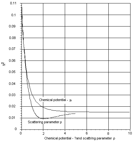 | Figure 3. Values of X2 as a function of the average scattering parameter and the chemical potential - µ of Fixsen’s model of equation 2.3 for the dipole radiation. For the scattering model the lowest value of X2 occurs at a temperature of 3.285843 oK and scattering parameter value of 2.0705567 for a value of X2 equal to 0.00932734686. For equation 2.3 given by Fixsen et al. the X2values asymptotically approaches a value of 0.015296145074 for very large negative values of the chemical potential and a value of 3.3301913 oK for the temperature |
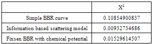
An attempt was made to calculate the optimum values of the temperature T and the chemical potential when the values calculated from equation 2.3 are compared to the dipole data of Table 2 using equation 2.1. The result of this is shown in Fig. 3. The value of X2 asymptotically approaches a value of 0.015296145074 for very large values of the chemical potential µ , see Fig. 3. Thus no unique value of the chemical potential µ could be obtained with this method. An optimum temperature of 3.3301913 oK was obtained.The IBM has the lowest value of X2 and is thus the best fit to the dipole data of the three models discussed here. Recall that the three models were the simple BBR curve, Fixsen’s BBR curve with chemical potential and the IBM. A comparison of models is listed in Table 3Table 3. Comparison of fit of models to data
 |
| |
|
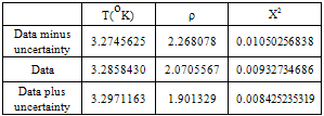
The interpretation of the dipole result differs from the one given by D. J. Fixsen et al. The interpretation here is that the dipole component of the radiation, unlike the radiation measured with a monopole instrument, is scattered before it reaches the detector.. The effect of the uncertainty in the data in Table 2 on the best fit temperature and scattering parameter are listed in Table 4.Table 4. Effects of uncertainty on data
 |
| |
|
A comparison of the normalized values calculated from equation 1.19 and the measured data of column 2 plus and minus the uncertainty of column 4 of Table 2 is shown in Fig. 4. The data in Fig. 4 is plotted as a function of the wave vector  in m-1.The explanation given here of the shift of the photon distribution to higher frequencies is doe to the effect of the scattering process as discussed above. This is a much simpler explanation than the one given by D. J. Fixsen et al. Thus by Occam’s Razor, perhaps the scattering explanation is the correct one?.
 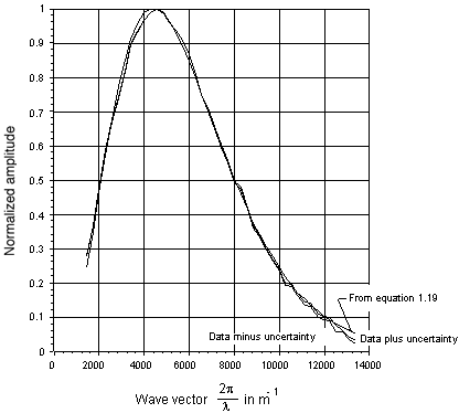 | Figure 4. A comparison of the normalized values calculated from equation 1.19 and the measured data listed in Table 2 as a function of the wave vector  . The three curves displayed above are the values calculated from equation 1.19 and the measured data plus and minus the uncertainty listed in column 4 of table 2. The calculated values are for a temperature of 3.28584 oK and a scattering parameter of 2.070585 . The three curves displayed above are the values calculated from equation 1.19 and the measured data plus and minus the uncertainty listed in column 4 of table 2. The calculated values are for a temperature of 3.28584 oK and a scattering parameter of 2.070585 |
The reason that the dipole radiation measured at the detector appears to be subject to scattering while the scattering parameter of the monopole radiation is equal to zero as well as the meaning of the value of the temperature of the dipole radiation source is left to wiser researchers than the author.
References
| [1] | “The Cosmic Microwave Background Spectrum from the Full COBE/FIRAS Data Set” by D. J. Fixsen, E. S. Cheng, J. M. Gales, J. C. Mather, R. A. Shafer, E. L. Wright, the Astronomical Journal, Vol. 473, pp. 576 - 587, 1996 December 20 1996. |
| [2] | “A Mathematical Theory of Communication” by C. E. Shannon, Bell System Technical Journal with corrections. Copyright 1948. Lucent Technologies Inc. All rights reserved. |
| [3] | “Probability Random Variables, and Stochastic Processes” By Athanasios Papoulis, McGraw-Hill Book Company New York London, ISBN 07-048448-1 (1965). |
| [4] | “Mathematical Models of Information and Stochastic Systems” by Philipp Kornreich CRC Press, ISBN 978-1-4200-5883-3 (2008) |
| [5] | “Analog and Digital Communication Systems” by Martin S. Roden, Prentice- Hall, Upper Saddle River N. J. 07458, ISBN 0-13-372046-2. (1996) |
 Abstract
 Reference
 Full-Text PDF
 Full-Text HTML