1. Introduction

The opportunity to find underground structures, such as fossil remains, is particularly stimulating forpalaeontologists, in order to work in wide areas, where the existence of those remains is just a hypothesis.

The GPR is a fast and cost-effective electromagnetic (EM) method which, in favourable conditions, i.e. mainly resistive non-magnetic environments, can provide valuableinformation on the shallow subsurface. Since it is based on the propagation and reflection of EM waves, it is sensitive to variations of the EM parameters in the subsoil, especially the dielectric constant and the electric conductivity[13]. Despite its relatively low penetration depth especially with high-frequency antennae and in moderately conductive environments), the GPR resolution capability (also depending on frequency and soil properties), by far greater than that obtained by other geophysical methods, makes this technique suitable for high-resolution shallow studies like archaeological applications and shallow stratigraphy mapping.

The advantages to use the GPR technique for the finding of underground structures of archaeological and geological interest have already been discussed by several authors[10, 11, 12, 15, 16, 17, 18, 19, 21]. The advantages of GPR for the finding of palaeontological remains, are less well known; in fact, very few authors have studied this question[7, 8]. Purpose of this work is to verify the effective GPR resolution capability in order to employ it for the location of palaeontological finds with consequent saving of excavation time and costs. With this purpose, some tests were carried out on biomicrite samples (with known position of the fossils).

The tests have been performed on:

◆ glauconitic biomicrite, which is a variety of the Pietra Leccese, with a fragment of Cetotheride maxillary (Cetacea-Mysticete) ;

◆ biomicrite with cetacean vertebrae (Scaldiceto);

◆ normal biomicrite with part of Psephophorus Poligonus (Chelonide);

The samples are dated in the Middle Upper Miocene.

Due to the samples thickness, both the 1000 MHz and 1500 MHz antennae were used[1, 2, 3, 4, 5, 20], with particular attention on the data acquisition (parameters and geometries of acquisition). Because of the small size of the targets, the data were acquired in very close parallel profiles (0.05 m). Subsequently the data were processed by means of 1D and 2D techniques and visualized in 3D space not only by the standard time slice technique, but also by iso- amplitude surface of the complex trace amplitude.

The use of 3D visualization techniques is of primary importance in palaeontological applications in order to display complex data in an easily understandable fashion, thus improving the quality and efficiency of the palaeontological interpretation. The most widespread way to display 3D radar data is in “time slice” (or depth slice) maps[11, 12]. Horizontal slices may not be the more suitable visualization technique in the case of great subsurface complexity since, for example, false amplitude anomalies can occur when the slicing planes cross dipping or undulating reflectors. However, time slices still remain the easiest and most rapid means to provide a synthetic view of the anomaly pattern, especially for large areas. For small-size zones a more complete understanding of the subsurface can be achieved by means of various 3D data presentations, including 3D cubes, chair views and slices parallel to the axes or along arbitrary directions. Interesting visualization approaches, involving the extraction and 3D visualization of the most promising signal attributes, have been proposed in recent papers[23, 24], where they have been successfully applied in imaging three dimensional bodies in mine detection and Non-Destructive testing applications.

The quick revealing of the spatial position of highly reflecting bodies, such as the anomaly related to the fossil remains in the tests on the samples, makes 3D visualization technique very attractive in palaeontological applications of GPR.

In the present study a trial of application of the 3D visualization techniques, along with classical time slice representation has been also made.

The results obtained from the different situations encountered in this work are very interesting. The satisfactory performance of the GPR method in the palaeontological research is confirmed.

2. Samples Description

The blocks investigated belong to two different varieties of Pietra Leccese, which is commonly represented by a biomicrite with calcareous cement, embedded in some places by thin marly levels.

The samples labelled A and B in Fig. 1 have been collected in the basin located near Maglie (LE), in the area stretching between Cursi and Melpignano.

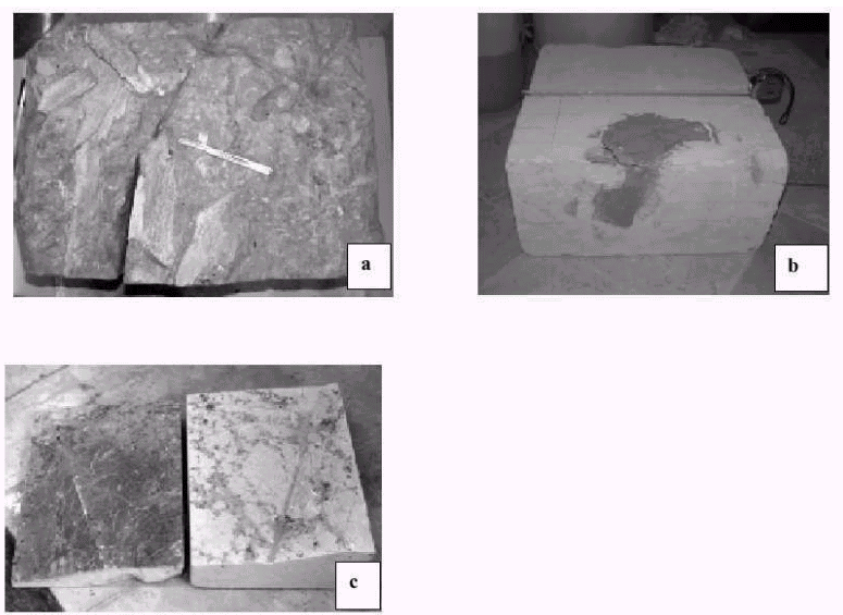Figure 1. Sample blocks: a) strongly glauconitic biomicrite (variety of Pietra Leccese “Piromafo”, containing a fragment of Cetacean maxellary (Misticete - Cetotheride); b)biomicrite containing Cetacean vertrebrae (Odontoceta-Scaldicetus); c) biomicrite containing a fragment of turtle carapace (Chelonide-Psephophorus)

Sample A comes from “Pietra Leccese” formation. It is afine sediment, basically made of planctonic foraminifera with carbonatic cement, and with a high percentage of glauconite (phyllosilicates from the illite group) and phosphatized elements. This particular sediment is known as “piromafo” , a Greek word indicating its resistance to high temperatures. In the block A is inglobated a fragment of Cetotheride maxillary (Cetacea- Mysticete).

Sample B was collected just below the piromafo level. It is a biomicrite showing the typical texture of “pietra leccese”: its colour goes from white to sub-white/yellowish, it is slightly more massive and weaker than piromafo. Its percentage of glauconite is very low and there are a few phosphorized elements. The block B contains few Cetacean Vertebrae.

Sample C in Fig. 1 has been collected in a quarry between Lecce and Cavallino. It is still the same biomicrite, but shows slightly different features: it is softer than sample C and is marked by the occurrence of highly diagenesized calcareous elements (nodules). The block includes a fragment of Turtle Carapace (Psephophorus).

3. Data Acquisition

Data acquisition is very important for a good geophysical survey. In fact, the acquisition parameters directly influence the data quality, and so all the following processing; therefore this choice must be very accurate and it must be done bearing in mind the aims of the investigation.

The choice of the antennae is equally important, because, as already said, the penetration depth and the GPR resolution capability depend on the electromagnetic pulse frequency.

Besides, it is necessary to remember that the different lithostratigraphical formation and physical features have peculiar effects on the radar sections[22] (reflection width and continuity, unity geometry, dominant frequency, diffraction presence and degree of penetration). Therefore, some preliminary measurements were made to estimate the best acquisition parameters. A reconnaissance survey was made in continuous mode, in a rectangular area along 0.05 m spaced parallel profiles.

4. Data Analysis

Block A

Block A, widely described in paragraph “Sample Description”, has the following dimensions: 0.4 m wide, 0.3 m high and 0.35 m thick. The fossil fragments lie at about 0.22 m in depth (Fig. 3a). The GPR survey was carried out in a rectangular area of 0.4 m by 0.3 m, along 0.05 m spaced parallel profiles using the 1000 MHz antenna in single-fold continuous mode (Fig. 3b).

The most accurate and straightforward method of estimating the EM wave propagation velocity in a medium, is to identify reflections in GPR profiles that are caused by objects of interest that occur at known depths. This method allows for a direct determination of the average velocity of EM waves from the surface antenna to a measured depth. The knowledge of both the block dimensions and the fossil remains position has allowed to estimate the average EM wave propagation velocity. In fact, the two – way travel time (t) from the surface to the fossil remains and back to the surface was measured at about 6.2 ns, and the measured depth (s) to the fossil remains was 0.22 m. The equation v=2s/t can be used to calculate the EM wave velocity in the block A which was 0.07 m/ns.

The quality of the raw data did not require advanced processing techniques. In fact only horizontal scaling normalisation and background removal filter have been performed for an easier interpretation. The application of the migration has not been particularly resolutive, since in the data there were nearly no diffraction hyperbolae. Consequentely, the migration has been omitted from the data processing.

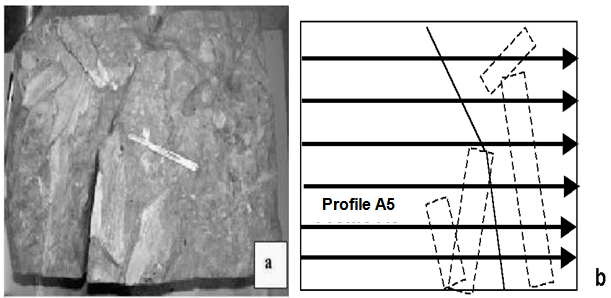Figure 3. Block A: a) photo; b) drawing of the side, with localization of the radar profiles and the fossil fragments

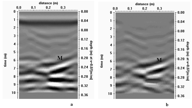Figure 4. Radar section relating to profile labelled A5 in Fig. 3: a) raw data; b) processed data

Figure 4 shows the reflection profile, labelled A5 in Fig. 3b. In Fig. 4, at time ranging from about 6.2 ns to about 10 ns (0.22 m - 0.35 m in depth), a reflection event is easily identifiable. Because of its high amplitude, denoting a strong electromagnetic contrast, this event was interpreted as due to the fossil fragments.

Due to the 1000 MHz antenna resolution capability, the single fossil fragments (about 2 cm size) did not underlined. Therefore, on the radar section (Fig. 4), only the anomaly concerning the group of fossil fragments has been obtained.

The processed data were then displayed with two different techniques whose main characteristics are briefly outlined below.

Time slice maps are built averaging the amplitude (or the square amplitude) of the radar signal within consecutive time windows of width Δt. Sometimes a particular complex-trace attribute, the instantaneous amplitude or envelope (modulus of the Hilbert transform), is used instead. Being a measure for the reflectivity strength, it helps evidencing high amplitude anomalies. Previous spatial averaging is also useful to reduce small-scale heterogeneity noise. Finally data are interpolated and gridded on a regular mesh[11, 12]. Selecting the various parameters involved[6] and in particular the width of the slice, Δt, is crucial. Typically Δt must be of the order of the dominant period, but different widths can be used in order to enhance particular features. In common practice, non-overlapping time windows are chosen, although sliding windows could be used instead, with the advantage of greater resolution but higher computational costs.

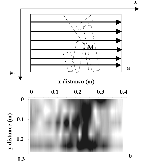Figure 5. Block A: a) drawing of the side, with localization of the radar profiles and the fossil fragments; b) time slices 6-8 ns

An approach for visualizing 3D radar data has been proposed by[24] for automatic mine detection. In this case, after an appropriate processing of radar data, a 3D image of the sought diffracting or reflecting object could be easily obtained by:

→extraction of the most promising complex signal attributes (trace energy and envelope);

→thresholding;

→3D contouring by means of iso – amplitude surface.

As pointed out by the authors, the threshold calibration is a very delicate task.

In Fig. 5 the time slice representations, using the absolute amplitude, are shown for block A, obtained using time interval of 2 ns (or approximately 0.07 m depth windows). A clear anomaly, 0.12 m long and 0.08 m wide, is visible on the 6 – 8 ns (0.21 – 0.32 m depth) slice.

In Fig. 6 the same data set is displayed with iso-amplitude surfaces using a threshold value of 50% of the maximum complex trace amplitude. Obviously, lowering the threshold value, increases the visibility of the main anomaly and smaller objects, but also heterogeneity noise. A relatively strong continuous reflection is visible on the 3D volumes (between 6 and 10 ns). In this case the anomaly related to the fossil remains is better emphasised. The threshold value selection is most delicate.

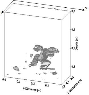Figure 6. Block A: 3D visualization by means of iso-amplitude surface of the complex trace amplitude using a 50% threshold. The anomaly related to the fossil remains is better emphasised

Block B

Block B has the following dimensions: 0.4 m wide, 0.2 m high and 0.2 m thick. The fossil fragments lie in the surface (Fig. 7a). The GPR survey was carried out in a rectangular area of 0.4 m by 0.3 m, along 0.05 m spaced parallel profiles using the 1500 MHz antenna in single-fold continuous mode (Fig. 7b).

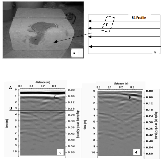Figure 7. Block B: a) photo; b) drawing of the side, with localization of the radar profiles and the fossil fragments; c) raw radar section relating to profile labelled B1; d) processed radar section

The EM wave propagation velocity in a medium has been calculated using the method that identifies reflections in GPR profiles that are caused by objects of interest that occur at known depths. This method allowed to estimate an average velocity of EM waves of about 0.12 m/ns. The quality of the raw data did not require advanced processing techniques. In fact only horizontal scaling normalisation and background removal filter have been performed for an easier interpretation. Figure 7c and d shows the raw reflection profile and processed reflection profile labelled B1 in Fig. 7b. An analysis of the Fig. 7d shows that:

● at time ranging from about 0 ns to about 3.4 ns (0 m - 0.2 m in depth), two reflection events are easily identifiable. These events were interpreted as due to the top and bottom of the block B respectively;

● at time ranging from about 0.4 ns to about 1.2 ns (0.024 m - 0.072 m in depth), a reflection event (labelled F) is easily identifiable. Because of its high amplitude, denoting a strong electromagnetic contrast, this event was interpreted as due to the fossil fragments.

The 1500 MHz antenna resolution capability, has emphasised the single fossil fragment.

The processed data were then visualized both in time slice maps and in a 3D iso – amplitude surface map.

In Fig. 8b the time slice representations, using the absolute amplitude, are shown for block B, obtained using time interval of 1 ns (or approximately 0.06 m depth windows). A clear anomaly, labelled F, is visible on the 1 – 2 ns (0.06 – 0.12 m depth) slice. This anomaly was due to the fossil fragments.

In Fig. 8c the same data set is displayed with iso-amplitude surfaces using a threshold value of 50% of the maximum complex trace amplitude. A relatively strong continuous reflection is visible on the 3D volumes (between 0.4 and 1.2 ns). Also in this case the anomaly related to the fossil rests is better emphasised.

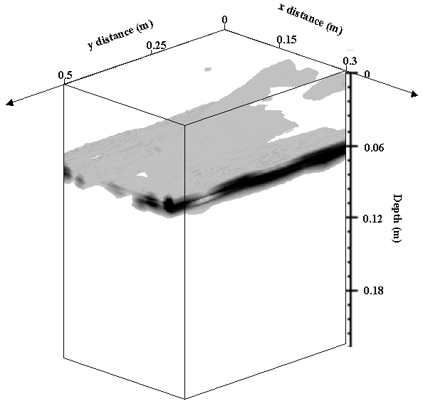
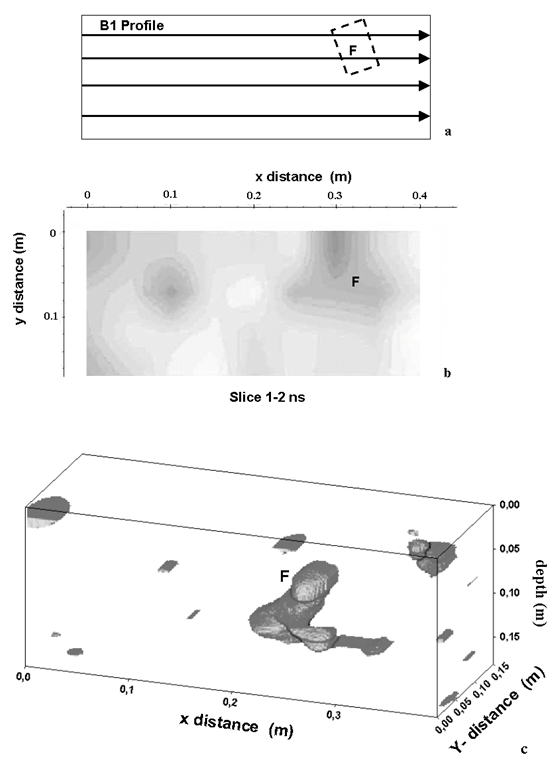Figure 8. Block B: a) drawing of the side, with localization of the radar profiles and the fossil fragments; b) time slices 1-2 ns; c) 3D visualization by means of iso-amplitude surface of the complex trace amplitude using a 50% threshold. The anomaly related to the fossil remains is better emphasised

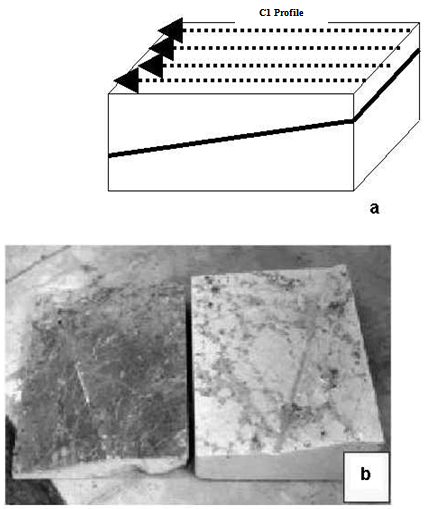Figure 9. Block C: a) photo; b) drawing of the side, with localization of the radar profiles and the fossil fragments

Block C

Block C has the following dimensions: 0.51 m wide, 0.4 m high and 0.18 m thick. The fossil fragments lie inside the block and it has a continuous and slightly inclined surface (Fig. 9a). The GPR survey was carried out in a rectangular area of 0.5 m by 0.4 m, along 0.05 m spaced parallel profiles using both 1500 MHz and 1000 MHz antennae in single-fold continuous mode (Fig. 9b).

The EM wave propagation velocity in the medium, was estimated to be about 0.12 m/ns. In this survey a further problem has been encountered: “the near – field effect”. An EM wave radiated from a surface antenna generates an EM field around the antenna within a radius of about 1.5 wavelengths of the center frequency[5, 14]. For the 1000 MHz antenna this effect is approximately 0.45 m if the EM wave radiates in air[11, 12], while it is approximately 0.18 m in the block C. For the 1500 MHz antenna this effect is approximately 0.3 m if the EM wave radiates in air, while is approximately 0.12 m in the block C. Within this zone, the EM wave is coupled with the ground, generanting an advancing wave front in the standard conical transmission pattern outside of the radius. It can be said that the ground within about 1.5 wavelengths of a standard dipole antenna is part of the antenna where no radiation is occurring within this zone, and therefore technically no propagation. In the GPR sections this zone is visible as an area of few or no reflections. To obviate the near – field effect zone a background removal filter was applied to all raw data.

Figure 10 shows the raw reflection profile and processed reflection profile (labelled C1 in Fig. 9b) related to the 1000 MHz antenna (Fig. 10 a and c) and the raw reflection profile and elaborate reflection profile related to the 1500 MHz antenna (Fig. 10 b and d). An analysis of the Fig. 10 reveals:

● for the 1000 MHz antenna, a very low correlation between the radar responses and the inclined trend of the surface, representing the fossil fragment. Even the processing carried out has not allowed to see the slope of the above mentioned interface (Fig. 10c);

● for the 1500 MHz antenna, the slope of the above mentioned interface is visible after the processing.

Time slice maps failed in imaging dipping events and therefore in this case were omitted.

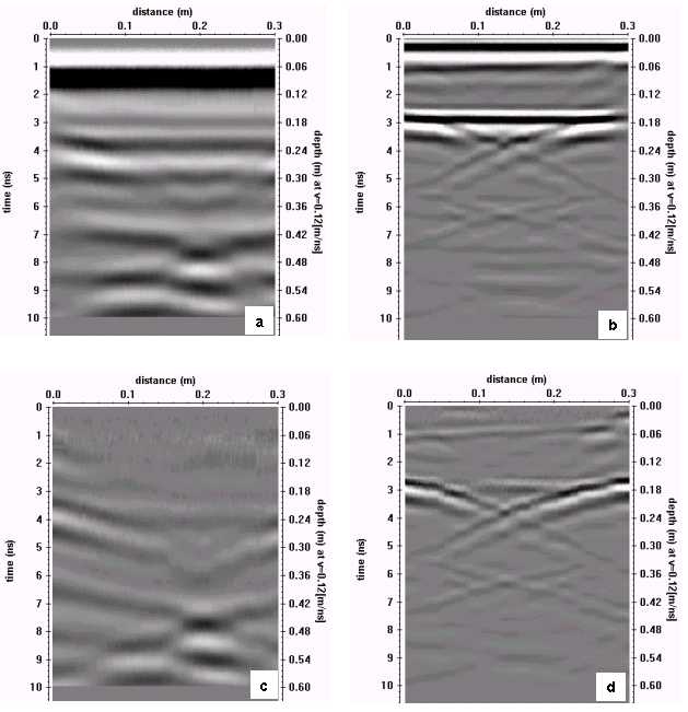Figure 10. Block C: a) raw radar section relating to profile labelled C1, obtained using the 1000 MHz antenna; b) raw radar section relating to profile labelled C1, obtained using the 1500 MHz antenna; c) processed radar section (1000 MHz antenna); d) processed radar section (1500 MHz antenna)

In Fig. 11 the same data set is displayed with iso-amplitude surfaces using a threshold value of 50% of the maximum complex trace amplitude. A relatively strong continuous reflection is visible on the 3D volumes (between 1 and 1.4 ns). In this case the anomaly related to the fossil remains is better emphasised.

Figure 11. Block C: 3D visualization by means of iso-amplitude surface of the complex trace amplitude using a 50% threshold

5. Conclusions

The geophysical investigation described in this work, aims to verify the potentiality of the GPR method to locate underground structures, such as fossil remains, at a depth of a few metres.

The response of the methodology, relating to the two units (blocks A and B-C) containing the fossil fragments has been very different: in fact, it mirrors the different electromagnetic and geolithological features of the investigated formations; inside blocks B-C, belonging to the same geolithological formation, the EM wave propagates without significant attenuation, while, inside block A the EM wave attenuation is slightly higher. This necessitates an accurate choice of the antenna; this choice is bound to the resolution, and so to the size of the structure to locate, and to the penetration depth.

However, the survey showed the presence of fossil remains inside the blocks investigated. Therefore, the technique offers a good response. Furthermore the primary importance of 3D visualization comes from the fact that it can provide a powerful and intuitive means of communicating complex information to non-geophysicists. Aside from the paleontological meaning of the features imaged, the present study allowed also a comparison of the performance of different visualisation techniques of GPR data.

Time slice maps, used mainly to enhance the horizontal relationships between amplitude anomalies, showed some alignments related to the fossil remains. Obviously this method failed in imaging dipping events as in the block C where there is an inclined surface that represents the fossil remains. They are more objective representation of the results than the other methods explored, but do not furnish an instantaneous view of the entire volume with the same immediacy.

The 3D contouring and isoanomaly plotting suffered from a certain degree of subjectivity in selecting the threshold value, but furnished very impressive pictures of 3D (and to a lesser degree also 2D or 1D) reflecting bodies, provided the data had a relatively high S/N ratio.

ACKNOWLEDGMENTS

The author wishes to thank Dr. Lara De Giorgi, for her useful co-operation during the data acquisition.