1. Introduction

Hillier and Hanson’s The Social Logic of Space[1] introduced the concept of space syntax and a suite of tools for the analysis of architectural and urban plans. The foundations of space syntax analysis originate in a field of mathematics known as graph theory that deals with the study of topological relationships. In order to apply graph theory to architecture, a range of mapping or abstraction techniques are required to convert complex spatial environments into a set of topological relationships. The three most common forms of abstraction, which precede analysis using space syntax mathematics, produce convex spaces, axial lines and visibility graphs.

The first of these three, convex space analysis relies on generalising an environment into a number of visually coherent spaces where a straight line drawn between any two points on the perimeter of a room will never intersect the perimeter in another location. Convex space analysis graphs and investigates accessibility; the configurational relationship between rooms as defined by the capacity to pass between them. Typically, environments such as architectural interiors, dominated by well-defined spaces, are the subject of this approach[2-5].

The second common space syntax method, axial line analysis, generalises environments into the set of the fewest and longest straight lines of sight and movement needed to survey or pass through a complete network of spaces. Axial lines represent idealised paths through space and the analysis of the topological relationships between axial lines is also an analysis of the movement potential of an environment. Axial line analysis is best suited to environments where long narrow paths prevail and it is commonly used to consider street configurations in urban districts. Axial line analysis also provides valuable insights into movement volume and potential at an architectural scale[6-9].

The third conventional method for generalising space is to create a visibility graph. This procedure imposes a regular grid over a plan of an environment and thereafter identifies the visibility relationships between each square in the grid. Depending on the input data, the analysis of these relationships reveals the visible (sight related) or traversable (movement related) properties of the space. This procedure almost certainly requires computational rather than manual analysis due to the relatively high number of calculations needed to analyse a space. Visibility graph analysis is best suited to well-defined environments such as those within buildings[10-12].

One disadvantage of convex space and axial line analysis is that their abstraction methods eliminate the opportunity to study precise locations in a plan. The former technique is effectively concerned with the properties of an entire room and the later with those of an access path. Visibility graph analysis suffers a similar problem, albeit to a lesser extent. The visibility graph’s ability to identify specific locations is subject to the availability of computing power and the resolution of the grid; a resolution of 500mm per grid line is common whereas a more accurate resolution of 100mm dramatically increases the number of calculations. Yet, architects often create spaces where particular locations are more significant than paths, rooms or general positions. For example, in a typical Romanesque cathedral the precise point where the axis of the nave intersects with the line of the chancel is both symbolically and phenomenologically important. Similarly, Le Corbusier’s vast orthogonal urban plaza in Chandigarh has neither defining walls nor clear paths, but it does possess a series of significant locations, often defined by the intersections between axes generated by elements in the space (like the Open Hand monument and the Tower of Shadows). While such cases are common in architecture, examples of designers discussing the spatial configuration of generalised rooms, paths or positions are, in comparison, rare. This suggests that, either there is a misalignment between the methods of designers and of analysts, or that new analytical techniques, to more rigorously interrogate the mathematical properties of specific locations, must be considered. It is the latter proposition, the need for techniques that can be focussed on points in space, that is the catalyst for the present paper.

Michael Batty[13] proposed an alternative approach to the social analysis of architectural and urban space which is reliant on an inverted version of the axial map; a process that shifts the emphasis of the map from the lines of movement or sight, to their intersections. Each of these intersection points is not only a precise location in space, but also the intersection of long lines of sight. Such points necessarily possess a relatively high level of both visual information and significance for way finding; both of which notably influence occupant behaviour[14, 15]. While this alternative method has potential for aligning the goals of designers and of building analysts, the mathematical processes may only be applied to the new intersection point graph if the data abstracted from the plan complies with the basic axioms of graph theory.

The present paper describes the development of an intersection mapping and analysis approach that allows for space syntax techniques to be used for the consideration of precise points on an architectural plan. The paper commences with an overview of graph theory and the differences between convex space, axial map and visibility graph analyses. Thereafter the paper describes a procedure for inverting the axial map and demonstrates, using three hypothetical villa plans, the construction of a valid intersection graph from an axial line map. Finally, the paper records the results of the mathematical analysis of one of these villas before offering concluding thoughts on the procedure and directions for future work. The detailed interpretation of these mathematical results is beyond the scope of the present paper although there are many examples available of how space syntax measures are used to understand spatial properties[1, 6, 16].

The analytical method described herein is a refinement of Batty’s[13] procedure for analysing the dual graph of an axial map. This procedure allows greater articulation of results than traditional axial line maps in locations poorly suited to visibility graph analysis.

While the method described in this paper has previously been suggested[13, 17], and some space syntax approaches relating to visibility graph analysis[10] do mathematically describe the properties of localised zones, the intersection analysis technique has not previously been demonstrated in this way. Furthermore, although Batty[13], and Jiang and Claramunt[17] have suggested urban applications of this approach, the potential architectural application has not been developed to a similar level of resolution, or described in detail, as the present paper does.

2. Background

The origins of graph theory may be traced to a topological puzzle centred on the Prussian city of Konigsberg which, in the thirteenth century, was a vibrant centre of commerce. At the heart of the city was the river Pregel, which “flowed around the island of Kneiphof[…] and divided the city into four regions connected by seven bridges: Blacksmith's bridge, Connecting bridge, High bridge, Green bridge, Honey bridge, Merchant's bridge, and Wooden bridge”[18 p200]. The puzzle challenges a person to identify a path through the city that shares a common start and finish point and crosses each bridge only once. Euler[19] proved that such a journey was impossible and, in doing so, developed a general theorem to solve similar problems by simplifying complex environments into a set of abstract relations. In this way, Euler’s theorem laid the foundations for graph theory; the formalised study of binary or pair-wise relationships between objects within a defined set. Such relationships, which are called topological, are described as binary because either a relationship exists or it does not.

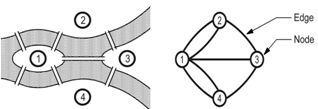Figure 1. A diagrammatic representation of Konigsberg’s geographic space (top) and a graph depiction of Konigsberg’s topological relationships (bottom) with locations represented by nodes and movement paths represented by edges)

In an architectural context, topological relationships describe rooms that are mutually adjacent (sharing one or more walls), or mutually accessible (sharing one or more doorways). These relationships require no metric data or further information although it is possible to ascribe additional values to them. The topological relationships in a system are typically represented diagrammatically in a graph (figure 1).

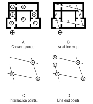
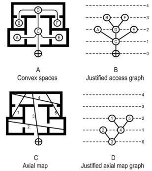Figure 2. (A) Plan view of a small villa identifying convex spaces, (B) that plan represented as the justified graph, (C) the axial line map of the same plan, and (D) its equivalent justified graph. Note: Axial line 3 (C) is node 3 (D) and incorporates the external carrier

Interest in graph theory grew from the mid 19^th Century, coinciding with the emergence of the modern representation of a graph as a node and edge diagram[18]. This type of figure abstracts spatial relations into a system of nodes connected by edges; in the case of Konigsberg these are, respectively, the landmasses and the bridges which connect them. However, there are several conditions that need to be fulfilled for a graph to be useful. First, a node may possess any number of edge connections but an edge can never connect more than two nodes. Second, it is possible for an edge to connect one node to itself creating a loop. This only occurs in a special type of configuration called a “multigraph” (figure 3-D). Finally, a further type of special graph, called “signed” or “biased”, can contain “half edges” that link a single node to nothing else. This last category of graphs is beyond the scope of the present paper.

Early examples of the application of graph theory to the built environment include analyses of accessibility and land use[20], transport networks[21, 22], facility planning[23] and building layouts[24]. However, it was Hillier and Hanson[1] who triggered the widespread application of graph theory to the built environment. Their research was soon expanded to include more detailed investigations of both urban[16] and architectural[6] cases.

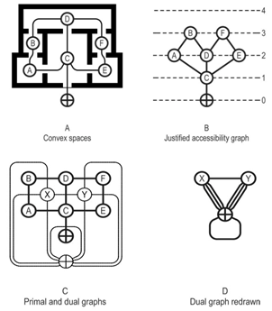Figure 3. A building plan (A) and associated justified access graph (B), form the basis of dual graph (C). The dual graph (the dotted lines in C) places a node in each region of the access graph with edges linking adjacent dual graph nodes (D). It is possible for a node in the dual graph to be adjacent to, and therefore link to, itself

One of the first approaches to spatial analysis that Hillier and Hanson[1] describe, convex space analysis, echoes the node and edge diagram of graph theory (Figure 2), with nodes representing rooms and edges representing doorways between rooms. A second approach, axial line analysis, begins by abstracting an environment to the fewest and longest straight lines that surveil all non-trivial spatial features[25]. These lines, both movement paths and lines of sight, become graph nodes and the intersections between the lines become graph edges (Figure 2). Once the graph has been constructed, it is then mathematically analysed to uncover the underlying spatial properties of the plan. Following the work of Hillier and Hanson, a range of scholars proposed refinements to the axial line method many of which focussed on developing stable and repeatable abstraction procedures to allow greater automation of the process[26-30].

From this point, the analysis is primarily of the graph and its mathematical properties, which can then be used to interpret corresponding features of the building plan it has been abstracted from. For example, the topological distance between nodes, measured in steps, can be calculated. A graph step occurs where an edge links two nodes, such that node F (Figure 2-B) is one graph step away from node D, and two steps distant from node B. Total depth (TD) is the shortest possible weighted step distance between one node and every other node in the graph whereas mean depth (MD) is the average weighted depth of a node relative to any other node in the graph. Another important value, integration (i), describes the accessibility of particular nodes relative to all others in the graph, and combined with the connectivity value provides a measure of plan intelligibility.

In practice, the mathematical values derived from convex space analysis are used to predict how people will use space, insofar as some spaces possess tendencies to promote concentrated use, while others are sufficiently isolated as to be unlikely locations of social interaction. This is because, as Bafna[31 p18] argues, the structure of society “is inherently spatial, and inhabited space has a fundamentally social logic”. In contrast, the results derived from an axial line map are thought to represent the spatial configuration of a plan, as experienced through movement[6], and visibility graphs indicate, amongst other things, locations from which large areas of the building are visible. From these methods of interpreting space, past studies have found that people exhibit particular behaviours while moving through a building or city. For example, Conroy[14 p208] observes that people in virtual environments “pause only in locations offering maximum visual, local/global information, reducing the necessity to pause more frequently” and that “people are pausing, in the main, at locations where a route choice decision needs to be made”[18 p139-140]. Thus, people do not move along axial lines in a regimented, mechanistic manner, rather these lines could be conceptualised as simply being connections between more important locations in space. Jiang and Claramunt[17] are also critical of the assumption implicit in axial line analysis that each path can be mathematically described as a singular experience. They argue that “the visual field observed from one end of a line is different from that observed from the other end of a line. More precisely, the visual fields from any individual standing points along an axial line are different. Thus, it is not logical to assign the same morphological properties to an axial line”[17 p301].

The axial line map could be regarded as suggesting that each sight-line or path has universal qualities, effectively encompassing all views simultaneously from every position on that path. However, a person moving along a path does not experience all views in all directions while in motion. In effect, their direction of travel constrains their cone of vision to what could be called “axial sight”; a 180° field of view that is required for collision avoidance. Moreover, the axial line intersection points are positions yielding the maximum amount of visual information and are concomitantly the decision points governing movement direction. At these ‘pause points’ the experience of space is more static, and a different type of 360° field of view, “intersection sight”, occurs. It is the obvious significance of these locations in space, for both way finding and movement, that leads Jiang and Claramunt[17 p301]to conclude that a “point-based approach” is clearly needed for architectural analysis.

Despite this argument, while axial line intersections approximate the pause points of inhabitants, in Conroy’s[14] research the correlation is not exact; pause points cluster around axial line intersections but do not perfectly coincide with them. This may be a result of the inability of occupants to physically achieve maximal visual distance due to the configuration of space or because occupants generalise the position of intersection points without needing to experience the optimal position. Furthermore, it is possible for the axial mapping process to produce two potentially valid axial lines for a single space, while only one is required for plan coverage[25]. These lines will possess identical length and connection properties, yet different geographic locations in the plan, and therefore, their intersection points are located in different positions. Because the decision on which line to include in the final axial map is based on an arbitrary, albeit universally consistent, protocol it is unreasonable to expect occupant pause points to perfectly mirror the intersection points on the map. Therefore, the proposition should be that axial line intersection points equate to idealised locations of maximum visual information and that occupant pause points approximate these locations.

3. Methodological Issues

Deriving mathematical values for intersection points requires these positions to be the subject of the analysis, which in turn requires an alternative representation of the axial map. Batty[13] refers to this alternate representation as the “dual” of the axial map; however, this term is a potential source of confusion. Graph theory researchers create the dual of a map by placing a node in each graph region and connecting these new nodes with edges that cross each edge in the original, “primal”, map (Figure 3). This procedure effectively makes each isolated set of walls the subject of the analysis, rather than the intersection points and is only applicable to planar graphs (Figure 4), yet most axial maps are not planar.

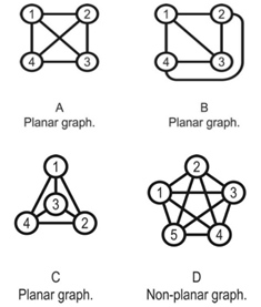Figure 4. A graph (A) which can have its nodes and/or edges rearranged in two-dimensions so that no edges cross each other while maintaining all topographic relationships (B and C) is planar. A non-planar graph (D) will always possess edges that cross, regardless of arrangement

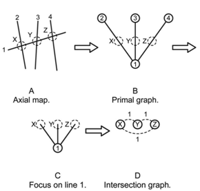Figure 5. Inversion of a simple axial map (A) to an intersection graph (D). (B) A justified graph of the axial map shows lines 1-4 as nodes and intersections X-Z as edges. (C) Focusing on axial line 1 shows that the node representing this line possesses three edges. (D) When the graph is inverted axial line 1 becomes a single edge and this edge is required to connect three nodes (previously intersections X-Z) which is impossible. Additional edges are therefore required to ensure all nodes are connected

Batty’s[13] procedure shifts the focus to intersection points by effectively inverting the axial map such that nodes and edges swap positions, a simple procedure where each axial line intersects fewer than three other lines. Inverting a map where an axial line intersects three, or more, other lines is problematic because each axial line becomes a single edge that is required to connect three, or more, nodes, which is impossible (Figure 5). To maintain the integrity of the axial map, every intersection point must be treated as if it is one topological step from each other intersection point of that line[13, 17]. In practice, this requires the introduction of additional graph edges to maintain the integrity of the map (Figure 6). A possible alternative approach is connecting only adjacent nodes, effectively increasing the total depth of nodes at the axial lines and decreasing the integration values of these positions. For instance, in the previous example (Figure 6), the far right node would be 3 steps from the far left node.

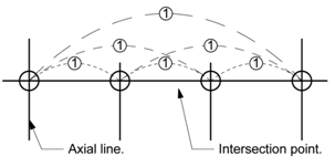Figure 6. All intersection points sharing a common axial line and the addition of additional graph edges ensure that each node is only a single topological step distant to any other node on the axial line

A further challenge in inverting an axial map is the decision of whether to include or exclude axial line “stubs”; that is, the portions of an axial line between the end of the line and its first intersection point. Excluding axial line stubs will focus the analysis of the inverted axial map purely on line intersections, the locations of maximal visual information. However, an advantage the inverted axial map offers a researcher is the ability to quantify the difference of spatial experiences at different locations along axial lines, including their ends. To study axial line ends, the stubs of axial lines must be included in the intersection graph.

The procedure for including line stubs in the intersection graph is simple; add a node to the end of each stub[13]. The procedure for excluding line stubs is even more straightforward; just ignore them. The difficulty arises from the fact that some line stubs are clearly more significant than others (Figure 7). Some line stubs contribute to plan surveillance or comprise the majority of an axial line’s length, while others are so short as to appear insignificant. An axial line intersecting only a single other line will consist entirely of two line stubs (Figure 7 line 2) and excluding line stubs prevents these axial lines from influencing the analytical results. These axial line stubs are required to describe the entire environment and a decision is required on which stubs to include in the mathematical analysis.

Figure 7. Lines 1 and 2 in the axial line map (B) are required to surveil convex spaces B and C of the plan (A). Axial line intersection points (C) fail to describe the entirety of the building configuration, whereas adding nodes D and E to surveil rooms B and C solves this problem

Turner[32] considers a similar problem when developing procedures for angular segment analysis. He suggests that the length of the stub, relative to the entire line, can be used to determine whether or not it remains in the analysis. Turner proposes “a segmentation routine that cuts off any stub of greater than, for example, 25% of the overall length of the line”[32 p148]. This suggests a classification system to define stubs, by percentage length, as long or short. Angular segment analysis excludes short stubs as being irrelevant and cuts long stubs from their parent line to create, and retain, new line segments. Turner goes on to state that “removing the stubs actually makes little difference to the analysis of the system”[32 p148] this, however, is due to the analytical focus on angular differences between line stubs. In a traditional space syntax approach, the decision to include line stubs is more significant. As Batty[13 p5] notes, “a street increases in importance as the number of nodes associated with it increases”. Therefore including stubs for some lines and not others increases the importance of some lines over others in the mathematical analysis.

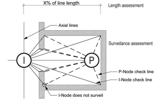Figure 8. Line stubs may be included in the intersection graph based on percentage length or surveillance assessments. P-Node check lines show the space surveiled, I-Node check lines pass through walls to meet the same surface vertex points thus the P-Node provides unique surveillance properties

Assessing lines entirely on length is potentially problematic because this cannot account for plan surveillance. Thus, a second procedure for use in conjunction with, or instead of, a length-based measure is required. Implementing selection based on plan coverage involves a simple, albeit laborious, process to determine if the end of each line stub possesses unique surveillance properties. This procedure mimics that for determining if axial lines contribute to plan surveillance[25]. The process commences by adding a potential node (P-Node) to the end of every stub then determining if each P-Node surveils a portion of the plan that no intersection node (I-Node) surveils. Surveillance is determined by drawing a straight ‘check line’ from each P-Node to each to each visible surface vertex (Figure 8). If an adjacent I-Node can draw similar check lines to each surface vertex associated with the P-Node, then that P-Node does not to contribute to plan surveillance. Nodes that provide unique surveillance properties are retained while those that do not are removed. The retained nodes may be relabelled as stub nodes (S-Nodes). It is also possible for multiple P-Nodes provide coverage of spaces with no I-Node surveillance; in such a case all P-Nodes are retained. The order of P-Node assessment does not affect the outcome of this procedure. Without a sufficient body of knowledge to suggest one approach is superior to another, it is acceptable to include all, some, or no stubs in the intersection graph provided the decision is logical and consistent where comparisons between applications are required. The resultant intersection graph is then analysed using standard space syntax procedures.

4. Worked Example

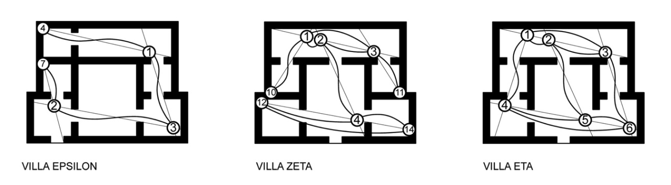
This section of the paper utilises the plans of three hypothetical villas to demonstrate a worked example of intersection point analysis. The villas form the basis of a previously published, extensively detailed, discussion on the creation of axial maps[25]. The authors designed each villa to possess identical footprints, a single external door and to produce a different type of axial map in each case (linear, branching or looping). The villas are named Eta, Zeta and Epsilon and six steps are required to develop the intersection graph from the axial line map and calculate the properties of each.

Step 1. Draw the axial map for the selected spatial configuration (Figure 9).

Step 2. Identify all axial line intersection points within the map and add an intersection node to these points (Figure 10) and assign each a unique identifier, in this case a numbered index.

Step 3. Select and apply a method for stub retention and removal (in this instance stubs are retained based on plan surveillance only). Begin by adding potential nodes (P-Nodes) to the end of every stub and assign a unique identifier to each (Figure 11). Determine if the P-Nodes surveil a portion of the plan that no I-Node surveils. Remove P-Nodes that do contribute to plan surveillance. Re-label retained P-Nodes as stub nodes (Figure 12).

Step 4. Map Inversion. During this step, the axial map is inverted to produce the intersection graph by linking I-Nodes and S-Nodes in a way that reflects the properties of the axial map. First, directly link each node associated with an axial line to each other node associated with that axial line. S-Nodes will only ever be associated with a single axial line whereas I-Nodes are always associated with two, or more, axial lines. The links ensure a graph step distance of one exists between every node located on a single axial line (Figure 13).

Step 5.Once the intersection graph has been produced, the axial map is no longer required (Figure 14) and, if desired, the intersection graph may be redrawn to clarify the topological relations although this has no impact on the mathematical analysis (Figure 15).

Step 6. Calculate the properties of each node following standard and widely-documented space syntax procedures as for any graph[1, 25]. These will begin with calculation of total depth, followed by the measures derived from this figure.

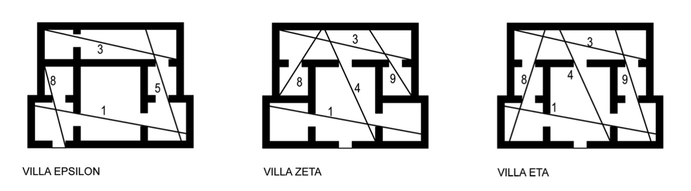Figure 9. Villas Epsilon, Zeta and Eta, and their axial maps, (Source: Ostwald and Dawes 2011)

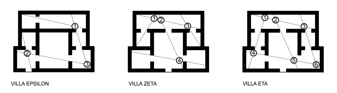Figure 10. Identification of intersection points and allocation of Intersection-nodes (I-Nodes)

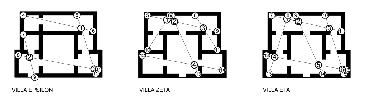Figure 11. Potential-nodes (P-Nodes) assigned to all stubs

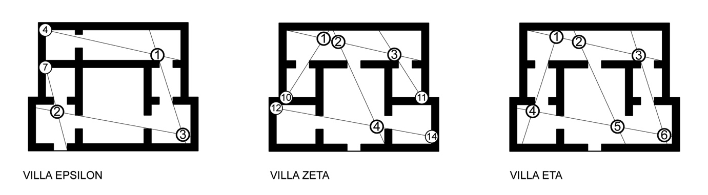Figure 12. Removal of P-Nodes possessing no unique surveillance properties; remaining P-nodes become Stub-nodes (S-Nodes). Villa Eta does not require S-Nodes

Figure 13. Addition of links to maintain character of axial map (shown dark and curved)

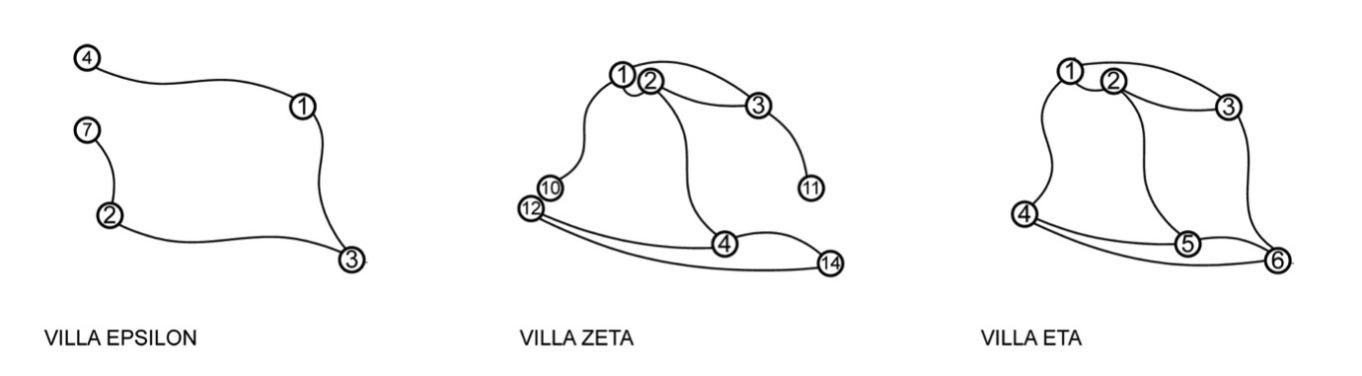Figure 14. Intersection graph of Villas Epsilon, Zeta and Eta

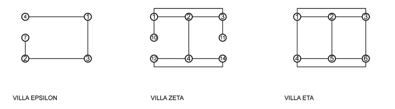Figure 15. Intersection graphs redrawn for clarity

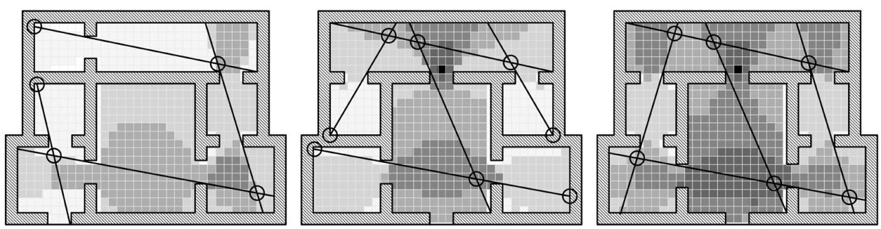Figure 16. Axial lines and intersection points for each villa imposed on a visibility graph analysis depicting high visual integration as darker tones

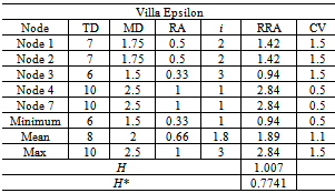
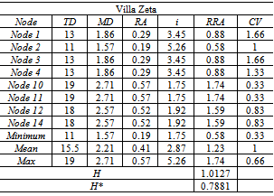
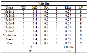
5. Results

The results of the mathematical analysis of the intersection points of each villa are recorded in Tables 1, 2 and 3. These results are especially informative when considered in the light of the other methods of space syntax analysis. For example, consider the results of a traditional visibility graph analysis for each villa with traditional axial map and intersection points superimposed (Figure 16). The visibility graph is shaded for visual integration values and it is clear that each axial line crosses a gradient of these values yet provides only a single measure for the length of this line.

Table 1. Intersection point analysis results for the Villa Epsilon

Table 2. Intersection point analysis results for the Villa Zeta

Plotting the values of the axial line and visibility graph analysis as a graph of the values encountered along the line shows that the traditional axial line measure (AX in Figures 17-19) remains static while the traditional, and computationally expansive, visual integration (VGA in Figures 17-19) experienced by an occupant varies considerably. Integration values of the intersection points (INT in figures 17-19) derived from the new method developed in the present paper, provide a greater degree of experiential articulation at a low computational cost. In the villas Epsilon and Zeta, for example, the values for the intersection points capture a degree of this variation while the particular spatial configuration of the villa Eta results in identical integration values for each intersection point. Therefore, the strength of analysing intersection points lies in considering those situations where axial lines do not provide sufficient articulation of spatial experiences and visibility graph analyses is restricted because the space is either too large (for fine scale analysis) or too ill-defined.

Table 3. Intersection point analysis results for the Villa Eta

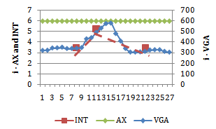
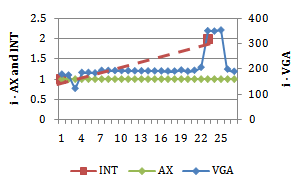Figure 17. Integration values for axial line (AX), intersection point (INT) and visibility graph analyses (VGA) as experienced by an occupant traversing line 3 in the villa Epsilon (moving from left to right)

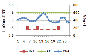
Figure 18. Integration values for axial line (AX), intersection point (INT) and visibility graph analyses (VGA) as experienced by an occupant traversing line 3 in the villa Zeta (moving from left to right)

Figure 19. Integration values for axial line (AX), intersection point (INT) and visibility graph analyses (VGA) as experienced by an occupant traversing line 3 in the villa Eta (from left to right)

6. Conclusions

This paper demonstrates a repeatable and rigorous procedure for analysing specific and significant locations in an architectural or urban plan, using the principles and practices of space syntax. This hybrid procedure combines lower computational needs (similar to the axial line approach) with the ability to analyse specific locations (similar to the visibility graph approach). Alternative variations of this method allow researchers to focus on particular areas of spatial interest such as locations of maximum visual information or evaluations of changes in spatial experience along the length of a single line of sight. Intersection points of long sight lines, locations of maximum visual information, become the subject of analysis using this method by excluding all axial line stubs from the graph. In contrast, including line stubs provides greater articulation of spatial experience and produces a different set of results during analysis.

Being an inversion of the axial map, the intersection graph is unable to capture information that has been “lost”, through abstraction, during the axial mapping process. For example, the axial map is unable to differentiate between the spatial experience of a long corridor and of an enfilade of spaces that are traversed by a single path. Without intersection points along this line, it is not possible for the intersection graph to differentiate between the experience of these very different spaces. This does not constitute a weakness in the intersection graph method because the intersection graph is a means of assessing locations that the axial map identifies as significant. The traditional convex space or visibility graph approach is therefore a more appropriate procedure for researchers desiring to evaluate every space in an environment.

Finally, the intersection graph procedure outlined in this paper suggests several future directions for research. First, while the intersection point mapping technique is derived from the process of inverting a more conventional axial map, a variation of this technique could be used to analyse the relationship between points in space identified by designers, or critics, as being significant for spatial experience. For example, as previously noted, Le Corbusier identified several important lines of sight across the grand plaza in Chandigarh, as well as multiple critical intersection points on this plaza. As Evenson notes, “[t]he generating motif of the [Chandigarh] complex, like that of the city itself, is a cross axis, but the arrangement of buildings is carefully plotted to avoid the static balance of rigid symmetry”[33 p72]. These important axes may operate as a substitute to axial lines however the mathematical analysis of these lines is unlikely to be informative and the area is too vast for visibility graph analysis. An analysis of the intersection and end-points of these axes, however, offers potentially informative results. Moreover, substitution of designed axes for axial lines becomes increasingly important in large open spaces where there are too few walls to create an unambiguous axial line map. Visibility graph analysis to identify specific and significant locations such as the intersection points of these axes is therefore unfeasible when utilising a human scale grid resolution both due to the sheer size of the spaces and to their lack of visual edges.

In addition to this possible use, for the method to be more widely applied, research must be undertaken to quantify the extent of mathematical differences between axial line maps and intersection graphs of typical spatial configurations and specific architectural contexts. Further research may then establish the significance of these differences by examining the correlation between mathematical measures and rates of spatial occupation. Finally, spatial occupation research could examine the impact of including or excluding axial line stubs and whether this change results in higher correlations to spatial occupation than predicted by standard axial line maps.

ACKNOWLEDGEMENTS

An ARC Fellowship (FT0991309) and an ARC Discovery Grant (DP1094154) supported this research.