1. Introduction

Multiphase fluid dynamics governs a wide range of natural and industrial processes, including inkjet printing, emulsification, spray cooling, and biological systems such as raindrop interactions and magma fragmentation. Accurate modeling of these complex flows requires numerical schemes capable of capturing interfacial Deformation, topological transitions, and phase interactions across multiple scales. The foundation for modern high-fidelity numerical methods was established by Patera [1], who introduced the spectral element method combining the flexibility of finite elements with the spectral accuracy of global polynomial expansions. This framework was expanded by Cockburn, Lin, and Shu [2], who developed the Runge–Kutta discontinuous Galerkin (DG) formulation for conservation laws, later refined for convection–diffusion systems by Cockburn and Shu [8]. High-order ENO and WENO shock-capturing schemes proposed by Shu and Osher [3,4] further improved the treatment of discontinuities while maintaining numerical stability and accuracy. Bassi and Rebay [7] extended these methods for compressible Navier–Stokes equations, enabling large-scale, high-order simulations.

The evolution of high-order numerical formulations continued with compact and Padé-type ENO schemes by Ma and Fu [10] and Wang and Huang [12], improving dispersion control and accuracy in wave-dominated flows. Subsequently, Liu, Vinokur, and Wang [17,18] formulated the spectral volume (SV) and spectral difference (SD) methods for unstructured grids, extended to multidomain three-dimensional Navier–Stokes solvers by Sun, Wang, and Liu [19]. These methods have collectively advanced the resolution and stability of computational fluid dynamics (CFD) solvers for multiphase flow problems.

Parallel to these developments, the lattice Boltzmann method (LBM) emerged as a mesoscopic alternative capable of simulating multiphase and multicomponent systems. The seminal work of Shan and Chen [5] introduced interparticle interaction forces to model phase separation and surface tension effects, while He and Luo [6] provided a rigorous theoretical framework linking the Boltzmann and lattice Boltzmann equations. However, subsequent models—such as Xing et al. [16], who proposed a perturbation-based single-phase surface tension model—imposed viscosity constraints that limited numerical stability. These challenges were later mitigated by Lee and Lin [15], who developed a stable discretization for incompressible two-phase flows at high density ratios.

Experimental studies by Gueyffier and Zaleski [13] and Cossali et al. [14] provided key insights into droplet splashing and coalescence phenomena, emphasizing the importance of Weber and Reynolds number interactions in determining collision outcomes. Complementary theoretical and numerical studies by Wang and Chen [9] and Succi [11] further reinforced the role of mesoscopic modeling in predicting complex fluid behaviors. By integrating these foundational advances, the present study leverages a sharp-interface LBM framework capable of resolving droplet deformation, Coalescence, and secondary breakup across a broad range of Reynolds and Weber numbers.

Finally, the incorporation of machine learning frameworks has transformed post-simulation analysis by enabling automated classification and prediction of droplet behaviors. Recent studies by Brunton and Kutz [20] and Yu and Chang [22] demonstrated the efficacy of physics-informed and data-driven models for understanding nonlinear flow regimes, while Bureš and Sato [21] applied sharp-interface phase-change models for evaporation and condensation. Building upon these advances, the present work integrates high-order numerical techniques with machine learning models—such as Random Forest, SVM, and XGBoost—to predict and classify droplet collision outcomes, bridging physical modeling with data-driven insight.

2. Numerical Methods

In this section, we describe the lattice Boltzmann formulation used to simulate sharp- interface multiphase flows. Our approach is based on the standard LBGK (Lattice Bhatnagar–Gross–Krook) model and incorporates a modified surface tension algorithm inspired by the Shan–Chen multiphase interaction model. This numerical framework enables simulations of high-density ratio systems, such as air–water flows, by improving interface stability and eliminating constraints on the relaxation parameter.

2.1. Lattice BGK Formulation

The evolution of the particle distribution function in the LBGK scheme is governed by the equation:

where:

• is the particle distribution function in the i-th direction,

• are discrete lattice velocities,

• is the relaxation rate,

• is the equilibrium distribution function.

The macroscopic density and velocity are recovered through the moments:

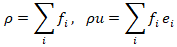The equilibrium distribution function used is:

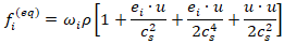where are direction weights and is the lattice sound speed.

2.2. Sharp-Interface Free Surface Assumption

Our model assumes that liquid and gas phases do not overlap; the interface is sharp and physically distinct. The gas density is treated as negligible, and its dynamic contribution is excluded from the simulation. The simulation tracks cell status—liquid, gas, or interface—by evolving the cell mass:

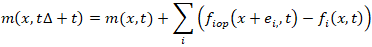Interface dynamics are managed by reclassifying cells based on mass thresholds. These updates enable dynamic interface reconstruction.

2.3. Modified Surface Tension Force

To enhance accuracy and stability, we incorporate a surface tension model as an external interfacial force based on Shan and Chen’s interaction framework. The original method by Xing et al. [16] introduced a perturbation function to the distribution functions but imposed a strict limit on viscosity and increased numerical complexity [16]. In contrast, our method applies a repulsive force between fluid and gas cells:

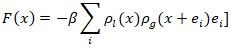where:

• is the liquid density,

• is a constant (representative) gas density,

• is a tunable parameter proportional to surface tension.

This force is applied only at interface cells where fluid and gas are adjacent. The post-collision velocity is modified as:

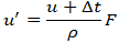This formulation allows for greater numerical flexibility by eliminating the viscosity limitation and enhancing stability at high Reynolds and Weber numbers.

2.4. Model Advantages

Compared to traditional methods, the proposed approach offers several advantages. In particular, the relaxation time τ is not restricted to values close to unity; it can be set to values greater than one, enabling stable simulations of high-viscosity fluids that are often challenging for conventional LBM formulations. Second, interface tracking is significantly more stable, owing to the implementation of a repulsive force formulation that enhances phase separation and reduces numerical diffusion. Lastly, the model robustly handles density ratios as high as 1000:1, making it well-suited for realistic air–water interactions commonly observed in multiphase flow scenarios. This improved numerical scheme provides a robust foundation for simulating droplet dynamics and collision phenomena, which are further explored in the validation and results sections.

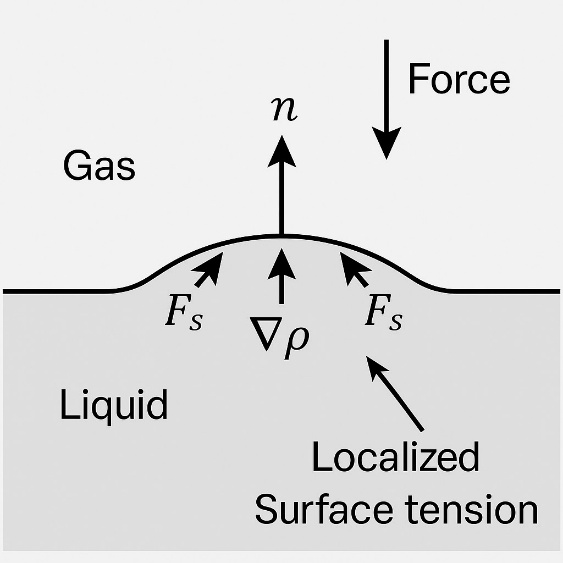Figure 1. Surface-tension layers and localized interface forces in the sharp-interface LBM formulation. Repulsive surface-tension forces act only on interface cells; the normal direction and density gradient are indicated. Concept follows the single-phase LBM force treatment where surface tension is applied as an external force in the collision step

2.5. Governing Equations and Dimensionless Parameters

Accurate simulation of multiphase systems depends on non-dimensional quantities that reflect the interplay between key forces. Three main parameters are used throughout this work:

• The Reynolds number quantifies the ratio of inertial to viscous forces:

where is the fluid density, is the relative velocity, is the droplet diameter, and is the dynamic viscosity.

• The Weber number represents the ratio of inertial forces to surface tension forces:

where is the surface tension.

• The Ohnesorge number represents the ratio of internal viscosity dissipation to the surface tension energy:

where is the surface tension.

• The impact parameter indicates the offset of colliding droplet centers:

where is the lateral distance between droplet centers.

3. Numerical Procedure and Results

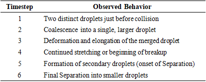
This chapter presents the results of numerical simulations performed using the sharp-interface Lattice Boltzmann Method, followed by validation against VOF results. To complement these findings, a machine learning-based classification of droplet collision outcomes is also introduced, leveraging data generated from the simulations.

In particular, we investigate and classify the dynamic behaviors that emerge during binary droplet collisions. These behaviors—stretching, Coalescence, Separation, and secondary droplet formation—represent the fundamental modes of interaction observed under varying flow conditions. Each regime is defined by the relative contributions of inertial, viscous, and surface tension forces, encapsulated in dimensionless parameters such as the Reynolds (Re) and Weber (We) numbers.

Stretching occurs when droplets deform into elongated shapes upon collision but remain connected, often forming slender liquid threads with larger bulbous ends. This regime is particularly sensitive to surface tension, which resists the breakup of the droplets and maintains their overall integrity. By contrast, Coalescence is characterized by the seamless merging of two droplets into a single, larger droplet, driven by surface tension’s tendency to minimize surface energy. In this regime, the fluid bridge between the droplets expands rapidly, creating a smooth, unified interface.

Separation arises when inertial forces dominate over surface tension, causing the droplets to rebound or split into three separate entities after impact. Finally, secondary droplet formation occurs when the collision energy is sufficiently high to fragment the droplets into four or more smaller droplets. This complex regime often involves both stretching and rupture dynamics, and it plays a critical role in understanding atomization processes, spray dynamics, and aerosol generation.

The results presented in this chapter provide a detailed examination of these four behaviors, revealing how variations in Re and We dictate the transition between regimes. The following sections guide the reader through high-fidelity simulations and visualizations of these outcomes, setting the stage for a deeper exploration of the underlying physics and the machine learning-based classification framework introduced in Section 3.3.

3.1. Numerical Results

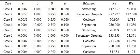
As illustrated in Figure 2, the fluid droplets exhibit significant viscosity and undergo noticeable stretching without fragmentation. The LBM simulation demonstrates a high degree of accuracy and numerical stability, with no visible discrepancies. These results highlight the robustness of the proposed algorithm in handling highly viscous flows, even with a relaxation time of .

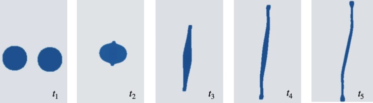Figure 2. Droplet stretching during a binary collision simulation with and The interaction occurs in a low-inertia regime, characterized by and , where surface tension dominates over inertial forces. The figure illustrates the maximum elongation of the droplets prior to the transition stage leading to Coalescence or rebound

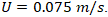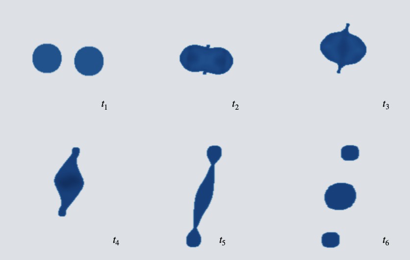
Figure 3 illustrates the formation of secondary droplets resulting from a moderate-velocity droplet collision, simulated under the conditions of and At this configuration, the flow exhibits a Reynolds number of approximately and a Weber number of placing the system near the threshold where inertial forces begin to overcome surface tension. As a result, the primary droplets deform upon impact and eject smaller satellite droplets, while the main fluid bodies remain partially intact. This regime demonstrates the onset of droplet fragmentation, driven by a balance between viscous resistance and capillary instability.

Figure 3. Formation of secondary droplets during a binary collision event with and The interaction occurs in a moderate-inertia regime, characterized by and where inertial forces begin to overcome surface tension, resulting in droplet breakup. The figure captures the moment of satellite droplet formation following the maximum elongation phase

As illustrated in Figure 4, the droplets undergo Coalescence under conditions characterized by a low Weber number and a reduced Reynolds number . This behavior is attributed to the combination of high surface tension and a low impact velocity which together suppress inertial effects and promote interfacial merging. Under these conditions, the capillary forces dominate, facilitating the Coalescence of the droplets without significant Deformation or breakup.

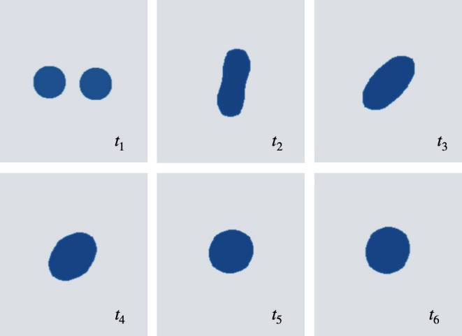Figure 4. Droplet coalescence during a low-inertia binary collision with and . The flow conditions, characterized by and , indicate a surface-tension-dominated regime where the droplets merge into a single continuous interface without the formation of secondary structures

Figure 5 depicts a droplet separation event under high surface tension conditions, with simulation parameters set to τ = 0.6, β = 10.0, U = 0.075 m/s, and D = 0.02 m. The resulting Reynolds number (Re = 2.5) and Weber number (We =0.011) are both notably low, indicating a flow regime dominated by viscous and capillary forces rather than inertia. Despite the strong cohesive forces induced by the high surface tension, the kinetic energy imparted by the collision is sufficient to overcome these forces locally, leading to the formation of distinct fluid bodies. The figure captures the subtle detachment process, where the droplet interface stretches and thins before separating into smaller segments, illustrating the complex balance between viscosity and interfacial tension in low-Weber-number collisions.

Figure 5. Droplet separation during a binary collision with and droplet diameter The conditions, defined by and correspond to a strongly surface-tension-dominated regime, where the droplets fail to coalesce and instead rebound after partial Deformation

These results show that higher Reynolds and Weber numbers lead to breakup and formation of secondary droplets, while lower values favor Coalescence or stretching. These trends are consistent with fluid dynamics theory.

To investigate the effects of different parameters on the simulation results, this study conducts 254 LBM cases.

3.2. Validation of the Numerical Model

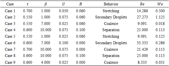
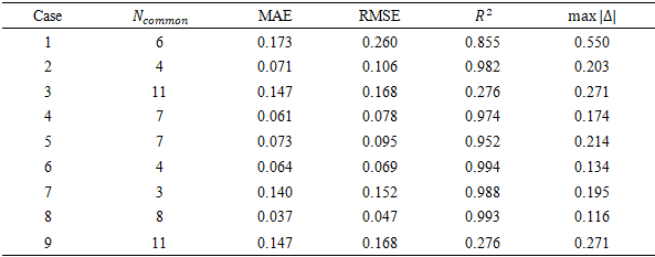
To validate the numerical approach, we first examine the mesh configuration and the ability of the model to capture the droplet interface. A refined mesh of 201 x 401 cells is used to ensure accurate resolution of the interface dynamics. We compare each of the frames of the images and record its behavior.

To verify physical realism, we compare LBM result frames with VOF results, as shown in Figure 6. Visual similarity is seen across behaviors in Table 1 such as Stretching and Separation.

Table 1. Observed Droplet Behaviors Across Sequential Frames

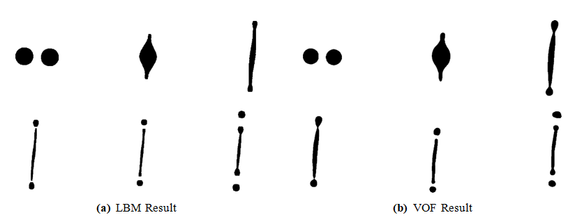Figure 6. Validation of droplet collision dynamics by comparing LBM and VOF simulations. The LBM result corresponds to with and 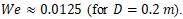The VOF result, using yields and The comparison demonstrates consistent droplet stretching behavior across both numerical frameworks

We conducted a comparative study of droplet–radius histories using two independent numerical solvers: LBM (SRT) and VOF. The analysis focuses on only nine cases, as detailed in Tables 2 and 3. To evaluate the agreement between the solvers, we computed the Mean Absolute Error (MAE), Root-Mean-Square Error (RMSE), and coefficient of determination using frames common to both solvers (Table 4).

Table 2. LBM (SRT) validation cases (1–9): material/flow inputs and resulting non-dimensional numbers

Table 3. VOF validation cases (1–9): material/flow inputs and resulting non-dimensional numbers

Table 4. Per–case agreement metrics between LBM (SRT) and VOF (common frames only)

The results demonstrate that LBM (SRT) and VOF produce nearly identical temporal trends, including extrema and relaxation rates. For Case 8, the strongest agreement between LBM (SRT) and VOF was observed (Table 4), with an MAE of 0.037, an RMSE of 0.047, and an of 0.993. Figure 7 illustrates this agreement through side-by-side plots of the dimensional radius (left) and normalized radius Both solvers capture the same time history, including the timing of the peak and subsequent relaxation, with only a modest amplitude difference at maximum Deformation. Normalization by further highlights the near-identical shape of the droplet evolution.

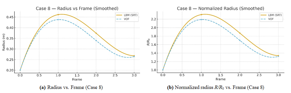Figure 7. Comparison of LBM (SRT) and VOF predictions for droplet radius in the best-performing case (Case 8). Left: dimensional radius in meters; Right: normalized radius R/R0. Both methods show close agreement (Table 4), with RMSE 0.037 and R2 = 0.993

To confirm that this agreement is not case-specific, Fig. 8 compiles normalized overlays for all nine cases. Most cases exhibit close alignment in the timing of extrema and relaxation rates, with occasional deviations (up to 10%) at frames of maximum Deformation. Cases with fewer overlapping frames (Table 4) appear sparser but adhere to the same trends. These findings indicate that LBM (SRT) and VOF consistently resolve the dominant droplet dynamics across all configurations, with residual differences likely attributable to model-form choices rather than significant numerical errors.

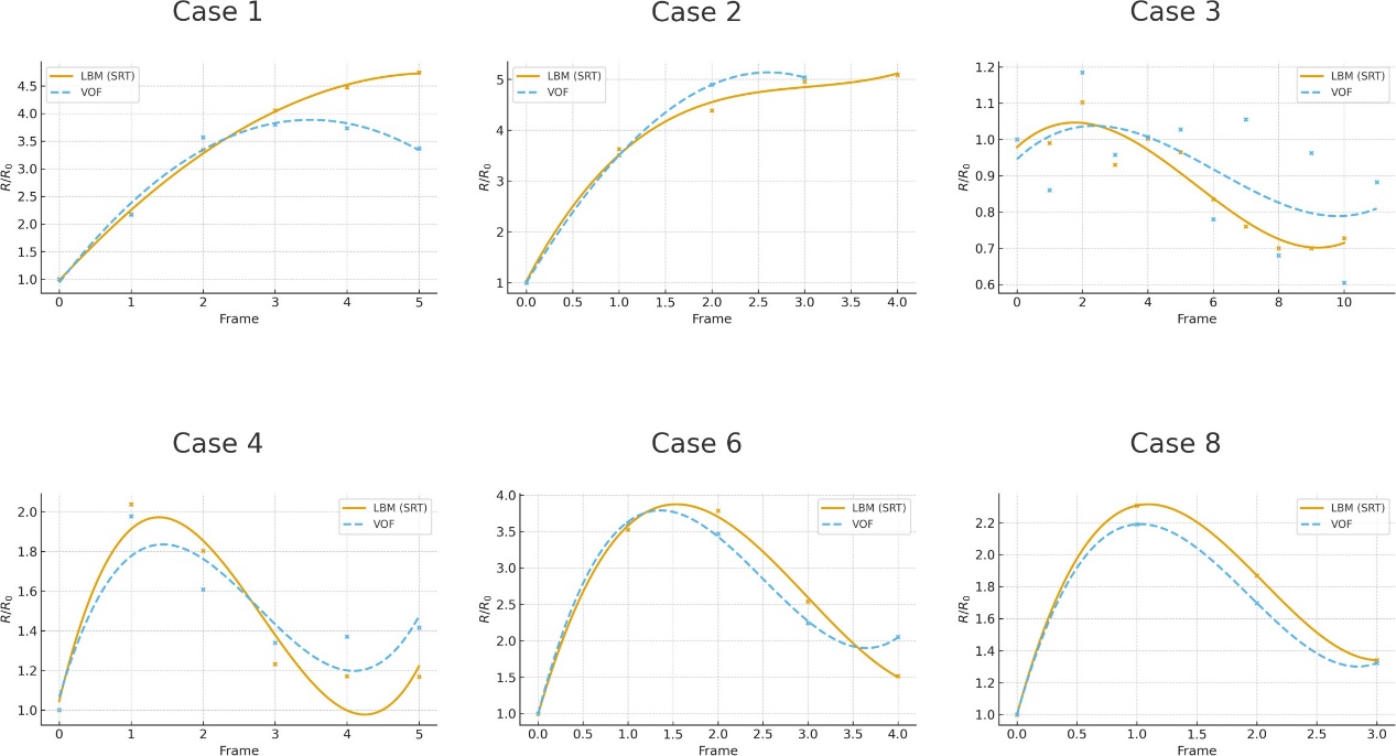Figure 8. Normalized radius R/R0 vs. Frame for best cases

This close case-by-case agreement indicates that both solvers effectively capture the dominant physical phenomena, including advection, capillarity, and viscous effects. The consistency across various model settings—such as meshing, time step, and collision/turbulence closure—reduces numerical and implementation uncertainties, thereby supporting the predictive fidelity of the chosen configurations.

While this study represents code-to-code corroboration rather than full experimental validation, the broad range of test cases and the strong normalized agreement provide a robust intermediate validation step. This justifies the use of these numerical models for subsequent analyses.

3.3. Machine Learning Classification of Droplet Outcomes

The purpose of applying machine learning in this context is to augment traditional fluid dynamics analysis by enabling fast, automated classification of droplet collision outcomes. While conventional simulation methods such as LBM provide detailed physical insight, interpreting the resulting behaviors across large datasets is time-consuming and subjective. By training classifiers on 254 simulations, we aim to identify key patterns and nonlinear relationships between physical parameters, as shown in Tables 5 and 6 and observed droplet behaviors. This data-driven approach not only accelerates post-processing but also enhances predictive capabilities, offering a scalable solution for analyzing vast parameter spaces and improving the interpretability of multiphase flow phenomena.

Table 5. Reynolds (Re) by behavior: median [IQR] and meanSD

Table 6. Weber (We) by behavior: median [IQR] and meanSD

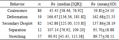
Table 5 summarizes the distribution of the Reynolds number across all observed droplet behaviors, providing a clear physical interpretation of how inertial effects influence collision outcomes. The results reveal that Coalescence occurs primarily within the lowest range (median = 45.45 [IQR 38.46–76.92]), indicating that viscous and surface tension forces dominate under these conditions, promoting the smooth merging of droplets. In contrast, Deformation exhibits the highest Reynolds numbers (mean = 162.68 ± 21.33), where inertial forces are sufficiently strong to overcome interfacial tension, resulting in significant droplet elongation or breakup. The secondary droplet regime also occurs at high Re values (mean = 137.86 ± 28.19), suggesting that instability at impact leads to satellite formation when inertia approaches or exceeds surface tension resistance.

Intermediate behaviors such as Separation (mean = 95.70 ± 18.88) and stretching (mean = 89.77 ± 38.51) occupy transitional Reynolds number ranges, where neither viscous nor inertial forces are entirely dominant. These regions mark the thresholds between stable Coalescence and unstable fragmentation, emphasizing the sensitive dependence of collision outcomes on inertia. The broad interquartile range observed in stretching behavior further indicates variability in droplet deformation patterns, often linked to minor variations in impact velocity or alignment. Overall, the Reynolds number statistics in Table 5 provide quantitative evidence that increasing inertia systematically drives the progression from Coalescence to deformation and secondary droplet formation, aligning with both experimental findings and the trends captured by the LBM simulations.

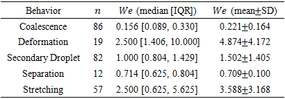
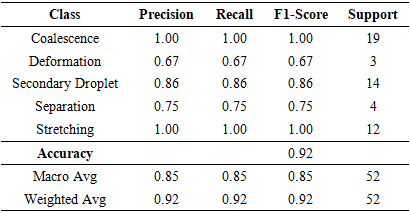
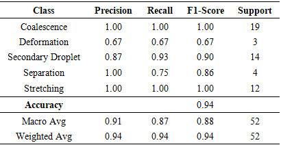
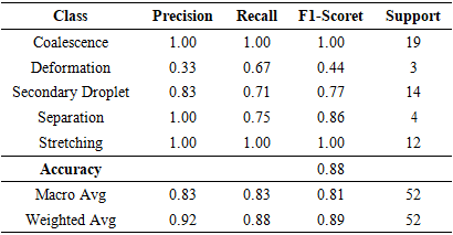
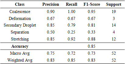
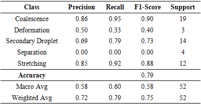
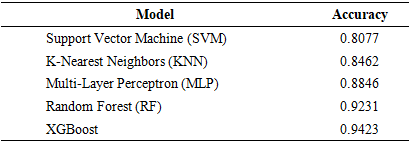
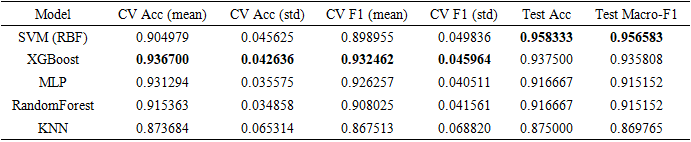
Table 6 presents the Weber number distribution for each droplet behavior, highlighting the role of surface tension relative to inertial forces during collision. Lower Weber numbers correspond to Coalescence (mean = 0.221 ± 0.164), where surface tension dominates and droplets merge smoothly without breakup. In contrast, deformation and stretching display higher Weber numbers (mean = 4.874 ± 4.172 and 3.588 ± 3.168, respectively), indicating that increased inertia overcomes surface tension, causing significant droplet elongation and transient instability.

The secondary droplet behavior appears in an intermediate Weber range (mean = 1.502 ± 1.405), suggesting a balance between inertial and capillary effects where breakup begins to occur. Meanwhile, Separation occurs at relatively low Weber numbers (mean = 0.709 ± 0.100), implying that droplets rebound rather than merge due to insufficient kinetic energy for Coalescence. Overall, these results demonstrate that as Weber number increases, the droplet behavior transitions systematically from stable Coalescence to Deformation and secondary droplet formation—consistent with the physical understanding of inertia-driven interface instability.

We used five models: Random Forest (RF), XGBoost, Multi-Layer Perceptron (MLP), K- Nearest Neighbors (KNN), and Support Vector Machine (SVM), as shown in Tables 7-11. Input features included Reynolds number, Weber number, impact parameter, and surface tension. Each model was trained on 80% of the data and evaluated on the remaining 20%. XGBoost and Random Forest achieved the highest accuracy among all models, as summarized in Table 12. Detailed class-wise metrics are shown in subsequent tables.

Table 7. Random Forest Classification Report

Table 8. XGBoost Classification Report

Table 9. MLP Classification Report

Table 10. KNN Classification Report

Table 11. SVM Classification Report

Table 12. Model Accuracy Comparison

3.4. Improving Machine Learning Model

We evaluated supervised models to predict droplet collision outcomes from primitive and dimensionless parameters. The evaluation set contained videos after the following preprocessing: (i) Separation was merged into Stretching; (ii) Deformation rows were removed as shown in Table 13; (iii) all numeric features were coerced, and rows with missing features were dropped. 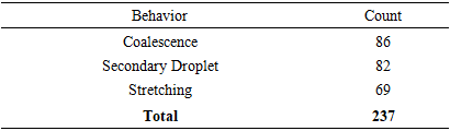Features included Viscosity, Surface Tension, Velocity Impact parameter (B), Density, Droplet Diameter, Reynolds, Weber, and Ohnesorge numbers. After preprocessing, the class counts were: Coalescence = 86, Secondary Droplet = 82, and Stretching = 69.

Table 13. Class distribution after merging, Separation→Stretching and removing Deformation

We trained Random Forest, SVM (RBF), KNN, MLP, and XGBoost using a pipeline with median imputation and (where appropriate) feature scaling. Hyperparameters were chosen from prior tuning; we performed 5-fold stratified cross-validation on the training split and selected the final model by test accuracy (macro-F1 as tiebreaker).

Table 14. Model comparison: cross-validation (CV) and test performance

As shown in Table 14, the cross-validation (CV) and test performance metrics reveal consistent trends across the five classifiers. The XGBoost model achieved the highest cross-validation accuracy (93.7%, 4.3%) and macro–F1 score (93.2% 4.6%), indicating excellent generalization during training. On the test set, however, the SVM with an RBF kernel outperformed all other models, attaining a test accuracy of 95.8% and a macro–F1 score of 95.7%. The Multi-layer Perceptron (MLP) and Random Forest models also performed competitively, both yielding test accuracies above 91%. In contrast, the K–Nearest Neighbors (KNN) classifier showed the lowest performance, with CV and test macro–F1 scores around 87%. These results highlight that, while XGBoost demonstrated strong cross-validation stability, the SVM generalized best on unseen data, a finding consistent with prior reports on classification tasks in fluid dynamics.

3.5. Trained Model Classification Performance

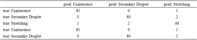
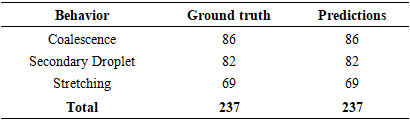
The confusion matrix shows only 6 misclassifications out of 237 as shown in Table 15. 4 boundary errors between Secondary Droplet and Stretching. 2 boundary errors between Coalescence and Stretching. These cases cluster in intermediate Weber numbers and moderate B (impact parameter), consistent with visually ambiguous outcomes near regime boundaries.

Table 15. Confusion matrix (evaluation set, N = 237)

The model’s high accuracy supports using Weber and B (with the other parameters) to screen operating points for desired outcomes. Near boundaries (e.g., moderate We and B), predictions should be paired with physical verification or higher-fps simulations. Merging Separation to Stretching simplifies the taxonomy and boosts performance; if Separation is required as a standalone class, the results produced reduced macro-F1 due to low support. Results reflect the current dataset’s parameter ranges; extrapolation outside these ranges should be treated cautiously.

Table 16. Class counts of ground truth vs prediction models

As shown in Table 16, the distribution of predicted behaviors matches the ground truth labels exactly across all three categories. Specifically, the model correctly identified 86 coalescence events, 82 secondary droplet events, and 69 stretching events, resulting in a perfect one-to-one correspondence with the true class counts. This consistency highlights the robustness of the trained classifier, indicating that the decision boundaries effectively capture the underlying regime transitions in the droplet collision dataset.

Table 17. Classification performance on the evaluation set (N = 237)

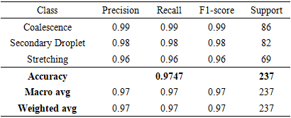
Among all evaluated models, the Support Vector Machine (SVM) with a radial basis function (RBF) kernel demonstrated the best overall performance on the evaluation dataset, achieving an accuracy of 0.9747 and a macro–F1 score of 0.974. The per-class metrics were uniformly high and well balanced, with Coalescence showing a precision, recall, and F1-score of 0.99 Secondary Droplet achieving 0.98 for each metric and Stretching reaching 0.96 across all three measures as summarized in Table 17.

4. Analysis of the Relationship Between Flow Inertia and Surface Tension

In this section, we utilize the trained machine learning model to investigate the intricate relationship between flow inertia, characterized by the Reynolds number (Re), and surface tension, quantified by the Weber number (We), in determining the evolution and outcomes of droplet collisions. Figure 9 presents the elliptical boundaries derived from statistical analysis, which clearly demarcate the transitions between distinct droplet behaviors, including Coalescence, Stretching, and Secondary Droplet formation. These boundaries serve as a visual representation of how the interplay between inertial forces, driven by fluid flow, and interfacial forces, governed by surface tension, dictates the regimes of droplet dynamics. The elliptical shapes in Figure 9 effectively map the Re-We parameter space, highlighting regions where specific droplet behaviors dominate, thus providing a comprehensive overview of the physical mechanisms that control droplet interactions under varying flow conditions.

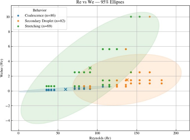Figure 9. Regime maps with decision boundaries classified by collision outcomes

Figure 10 complements this analysis by showcasing the classification boundaries established by the machine learning model, specifically a Support Vector Machine (SVM), for droplet collision outcomes as a function of Re and We. The SVM model delivers a significantly more refined and meticulous classification compared to the statistical boundaries presented in Figure 9. By capturing the nonlinear relationships between inertial and surface tension forces, the SVM delineates precise regions in the Re-We parameter space where distinct outcomes, such as full Coalescence, partial stretching, or secondary droplet formation, occur. This enhanced resolution underscores the strength of machine learning in resolving subtle variations in droplet behavior that may be overlooked by traditional statistical methods. The classification boundaries in Figure 10 not only highlight the dominant regimes but also reveal the sensitivity of droplet outcomes to small changes in Re and We, offering a deeper understanding of the complex dynamics at play.

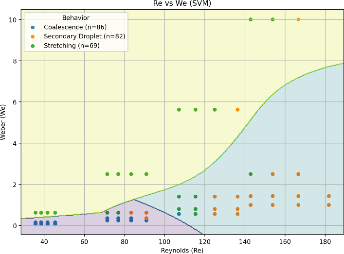Figure 10. Support Vector Machine (SVM) classification boundaries for droplet collision outcomes in the Reynolds number (Re) versus Weber number (We) parameter space

To further enhance the physical interpretability of the machine learning results, we examine the relative contribution of each input variable to the classification decision-making process. Figure 11 presents the feature importance scores computed from the trained Random Forest model. The Weber number and Reynolds number are identified as the dominant predictors of droplet collision behavior, confirming that the balance between inertial and surface tension forces governs regime transitions. Surface tension viscosity and impact parameter also contribute, though to a lesser extent, indicating their secondary roles in refining boundary distinctions between stretching, coalescence, and secondary droplet formation. These results align with the physical understanding of droplet impact processes and provide transparency to the machine learning model’s internal decision structure.

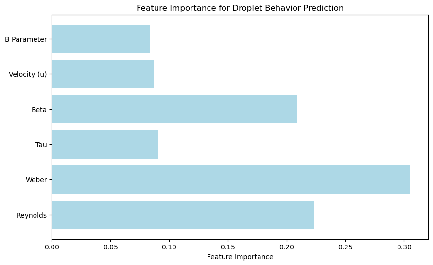Figure 11. Feature importance ranking from the Random Forest classifier used to predict droplet collision outcomes. Weber number (We) and Reynolds number (Re) dominate model decision-making, indicating that the classification strongly reflects the underlying balance of inertial and interfacial forces governing droplet behavior

5. Conclusions

This study presents a comprehensive investigation of the lattice Boltzmann method (LBM) and its governing parameters, with direct comparisons to the Volume of Fluid (VOF) method under equivalent physical conditions. By incorporating a modified surface tension model and transferable velocity formulation, we developed an enhanced LBM framework capable of accurately reproducing five key droplet collision behaviors: stretching, Separation, secondary droplet formation, Coalescence, and Deformation. The simulations demonstrated that the proposed model successfully captures the dynamic transitions among these behaviors, revealing distinct Reynolds and Weber number ranges associated with each regime.

To validate the LBM framework, nine cases with matched parameters were simulated and compared against corresponding VOF results. The radius evolution curves exhibited strong agreement between both methods, confirming the physical consistency of the LBM predictions. These findings were further supported through analysis of dimensionless parameters, where both the and values followed comparable trends across the two approaches.

Statistical analysis of the simulation dataset indicated that merging the separation and stretching behaviors improved the robustness of classification outcomes. Using these refined categories, we trained multiple machine learning models and achieved high predictive accuracy, with the SVM (RBF kernel) model attaining 97% accuracy and balanced class performance across behaviors. Finally, the trained model was applied to explore the relationship between flow inertia and surface tension in determining droplet collision outcomes. The resulting elliptical regime maps clearly delineate behavioral boundaries, offering deeper insight into the transitional physics governing multiphase droplet interactions.

Overall, this research demonstrates that the sharp-interface LBM approach, combined with machine learning-based classification, provides a robust and data-informed framework for studying droplet dynamics and validating multiphase flow behaviors with high fidelity.

ACKNOWLEDGEMENTS

The author gratefully acknowledges the support of the Bridge to Academia Fellow Program through Virginia Tech for funding this research. Their investment in fostering academic scholarships and advancing computational science provided the resources and guidance necessary to complete this work.

Data Availability

The datasets generated and analyzed during the current study are not publicly available due to project and storage limitations, but they are available from the author upon reasonable request. Interested readers and researchers may contact the corresponding author to obtain access to the data supporting the findings of this work.