-
Paper Information
- Paper Submission
-
Journal Information
- About This Journal
- Editorial Board
- Current Issue
- Archive
- Author Guidelines
- Contact Us
Applied Mathematics
p-ISSN: 2163-1409 e-ISSN: 2163-1425
2022; 12(1): 8-16
doi:10.5923/j.am.20221201.02
Received: Feb. 8, 2022; Accepted: Mar. 7, 2022; Published: Mar. 28, 2022

Source-to-Sink Distribution in a Feasible Autorhythmic Volume Conduction System
 Abstract
 Reference
 Full-Text PDF
 Full-text HTML
Nzerem Francis Egenti, Ukamaka Cynthia Orumie
Department of Mathematics and Statistics, University of Port Harcourt, Nigeria
Correspondence to: Nzerem Francis Egenti, Department of Mathematics and Statistics, University of Port Harcourt, Nigeria.
| Email: |  |
Copyright © 2022 The Author(s). Published by Scientific & Academic Publishing.
This work is licensed under the Creative Commons Attribution International License (CC BY).
http://creativecommons.org/licenses/by/4.0/

Sources and sinks are phenomena of interest. Biological systems have their share of the inherent benefits derivable from them. One of such systems is the Autorhythmic Volume Conduction System (AVCS). Autorhythmicity is typical of electrically active cells that demonstrate rhythmic activity without being driven by external stimulation. It is a unique attribute of cardiac cells. Here, specialized nodal cells act as sources and sinks, with the conduction pathways maintaining the integrity of ionic flow. The edge-nodal system is a network. Feasible network flow of ionic current is often achieved by the synergy between edge-nodal appurtenances. A veritable way of analyzing network systems is the mathematical graph theory. Therefore, this was done here. Much as the AVCS has its idiosyncrasy in terms of current flow through edge-nodal structures, the analysis of electrical flow as evinced by source and sink phenomena is a clue to a better understanding of the conduction system of the heart.
Keywords: Bioelectric, Graph theory, Network, Impulse, Action potential, Maximize
Cite this paper: Nzerem Francis Egenti, Ukamaka Cynthia Orumie, Source-to-Sink Distribution in a Feasible Autorhythmic Volume Conduction System, Applied Mathematics, Vol. 12 No. 1, 2022, pp. 8-16. doi: 10.5923/j.am.20221201.02.
Article Outline
1. Introduction
- Bioelectric phenomena predate all artificial forms of electricity. In bioelectricity endogenous electrically mediated signalling regulate cell, tissue, and organ-level modelling and behaviour. Cells and tissues of all types, in the main, use ion fluxes to communicate electrically. Bioelectric phenomena are usually described by volume conduction models. Such models describe the topology and conductivity of tissues wherein electric current flows and also the current sources in the tissue. The heart is typical of an autorhythmic volume conduction system, and it is therefore being considered here. It is here named autorhythmic volume conduction system (AVCS). Autorhytmicity is a unique attribute of cardiac muscle cells. The cells can generate an autonomous action potential (AP) to an enormous degree.The passage of ionic current across the membrane of active excitable cells induces sources and sinks. In the AVCS the nodal structures, which include the sinoatrial node, atria, atrioventricular nodes (AVN), His bundles, Purkinje’s fibres act as electric sources and sinks. The heart is a site for the transmission of autonomous and automatic AP. The propagation of such APs is contingent on the efficient conduction of electrical current from an excited cell to an abutting quiescent cell. Sources and sinks are created when cells give charge to abutting quiescent cells. Almost every cell in the AVCS acts as a source and a sink. The source-sink balance is an essential issue in the cardiac system. In this regard, Unudurthi et al. [1] depicted the pivotal role of the sinoatrial node (SAN) in the integrity of cardiac source-sink balance. Nikolaidou et al. [2] showed the elegant source-sink relationships that reside in the SAN region. The consummation of the conduction system presupposes the generating of the quantity of current that would be sufficient for the local sink. This is one possible way of avoiding source-sink mismatch which is largely implicated in the deleterious cardiac events. The choice of the term feasible in the caption of this work implies a mismatch-free dipole. In this regard, Boyle and Vigmond [3], Kleber and Rudy [4] stressed safety needs and therefore the quantification of the source-sink balance. The question of how specialized cells prosecute, nay, control the conduction system given their susceptibilities requires great attention. For instance, how does the relatively small SAN cope with the electrical exigencies of the much larger atrial tissue? Such a source-sink mismatch is also seen in the Purkinje fiber–ventricular junction where a small Purkinje fiber (source) is coupled to a large mass of ventricular tissue (sink). How do the Purkinje cells satisfy the ventricular mass to cope with a source-sink mismatch? To be quite succinct, one may read what Joyner and Capelle [5] say as regards the earlier question, and see Morley et al. [6] for the latter question. We are yet to define the conduction network or, if you like, pathway: This is sequentially made up of the SAN, the atrioventricular node (AVN), and the His-Purkinje system. The anatomy of each of the above, which is not within the scope of this work, may be found in numerous Anatomy and Physiology works of literature including Monfredi et al. [7] and Kurian et al. [8]. Cardiac myocytes are connected end to end by intercalated disks. Adjacent to the discs is the gap junctions. Of physiological and electrical importance are the low resistance gap junctions. These junctions allow APs to spread from one myocyte to the next. They decisively determine how much depolarizing current passes from excited to quiescent regions of the network. Thus, they determine the speed and safety of the conduction process [9]. Gap junctions are known sites for electrical coupling between cells. Woodbury and Crill [10] supplied a treatise on electrical potential at the gap junction between two contiguous cells way back in 1970. Writing in contemporaneous times with the former, Heppner and Plonsey [11] produced a seminal work on the electrical interaction of cardiac cells. In real cardiac tissue, however electrical conduction takes place in both the intracellular and extracellular space in cardiac tissue, wherein there are variations in conductance and anisotropic ratios. Heppner and Plonsey [11] considered the intracellular and extracellular media as passive volume conductors of longitudinal resistances.At present, mathematical treatment of the cardiac source-sink process is sparse in literature. A detailed understanding and application of graph theory [12,13,14] seem invaluable in the study of the AVCS. This work took this reasoning into account; it presents a mathematical approach to the understanding of the AVCS mechanism which is anchored on cell-to-cell source-sink electro-physiological flow. The issue of cell-to-cell flow here was treated as a network problem (see Rubido et al. [15,16], Wang and Lai [17], and Ahuja et al. [18]).
2. Graph Theoretics of the Source-Sink Network
- Let G = (V, E) be a directed graph (digraph), where V and E are the node (vertex) set and segment (edge) set respectively. Let N = N(s, t) be a network, with two distinct vertices- a source s and a sink t, together with a non-negative real-valued function c defined on its arc set A. The vertex s corresponds to a production centre, or in the present case the impulse generating node, and the vertex t to a consumer, or the adjoining impulse receiving node. The function c is the capacity function of N and its value on a segment l is the capacity of l. The capacity of a segment may be seen as the maximum rate at which a substance can be transported through it.An (s, t)-flow in N is a real-valued function f defined on a set S such that
 | (1) |
 | (2) |
 | (3) |
 | (4) |
2.1. Graph Metrics
- Graph metrics reveal the diverse characteristic of a defined network. Some salient ones are as follows:
2.1.1. Integration Metric
- This estimates the relative ease with which cell regions communicate. If vi and vj are two adjoining nodes then the Shortest Path Length (SPL) between them is the shortest path that reaches vj beginning from vi. It is the shortest number of edges between vi and vj; for a weighed graph SPL is the sum of all the edge weights in the shortest path between vi and vj, calculated as
 | (5) |
 The global efficiency of the graph is calculated as
  | (6) |
2.1.2. Segregation Metric
- This measures the presence of clusters or modules within the network. Modularity is the degree to which a network may be partitioned into prominently delineated and non-overlapping groups. We may not bother much about the intricacies of this metric since the network in this study is not as complex as to require its use.
2.1.3. Measure of Centrality
- Degree centrality is calculated by counting the neighbours of each vertex. It is given by
 | (7) |
 | (8) |
 | (9) |
 | (10) |
2.1.4. Measure of Resilience
- This is a metric of the vulnerability of the network as regards functional integration.
2.2. Impulse Transmission on the Conduction Network
- The graph G = (V, E) here is treated as analogous to an electric network. Kirchhoff’s flow network is ideal in the treatment of minimal cost in transportation, including biological steady-state systems. We assume that the flow network obeys Ohm’s law. Thus,
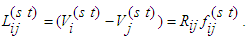 | (11) |
 represents voltage drop across the segment (i→j) connecting nodes at i and j, with a source situated at node s and a sink situated at node t. The segment (i→j) has a resistance Rij against the flux fij which is determined by the conductance of the segment l. By conservation condition (11), the net flow at any node in the network must vanish. Therefore,
 | (12) |
 | (13) |
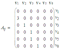
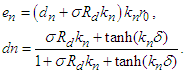
2.2.1. Constructing the Adjacency Matrix of the AVCS
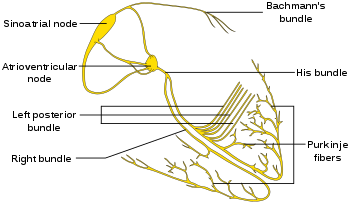 | Figure 1(a). Electrical conduction system of the heart [23] |
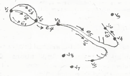 | Figure 1(b). Node-edge schematic of the CCS [24] |
 | (14) |
 | (15) |
 | (16) |
 | (17) |
 | (18) |
 | (19) |
 | (20) |
3. Ionic Flow and Action Potential
- Like biological fluid-structure interaction problems [25], the cell-to-cell flow consists of the cardiac cellular structures and the ionic substances in current. However, unlike the Eulerian formulation that characterizes fully developed fluid flow, the present flow is amenable to Kirchhoff’s laws. The treatment of general cardiac APs is somewhat herculean due to variations in the constitutive ions and APs of the various cardiac myocytes. It would seem rather plausible to treat conduction in cell-to-cell segmentations, thereby accommodating their idiosyncratic APs (see Qu et al. [26]). In the AVCS, the electrical impulse is generated in the SAN, which spreads quickly through the atria to the atrioventricular node (AVN). (Note that the SAN is electrically coupled to the atria). The impulse travels from the AVN to the His-Purkinje system. Eventually, the Purkinje fibres transmit the impulse to the ventricular muscles at numerous discrete locations. The problem of source-to-sink distribution involves triggering an AP in a quiescent cell by an abutting active cardiac cell. The architecture of a cardiac strand, with its many individual cells of irregular shapes, is a mathematical task. Here each cell is assumed cylindrical and non-tapering.
3.1. Bidomain Electrical Flow
- Bidomain structure defines a model of the heart tissue comprising two interpenetrating domains representing cardiac cells and the surrounding space, the intracellular and the extracellular domain [27,28]. The continuous topology of the intracellular space enhances ion travel from the inside of one cell to another via gap junctions without getting into the extracellular space, nor would ion travelling in the extracellular region require entry to the cell. Both spaces have electrical autonomous properties, therefore they form an anisotropic medium. Let the associated internal and external potentials of the domains be
 and
and  . Then the transmembrane potential is
  . The current associated with the internal and external potentials are
  and
and  respectively. By Kirchhoff law
 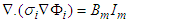 | (21) |
 | (22) |
 | (23) |
 | (24) |
 is the cardiac domain, n is the outer unit normal vector to the boundary
  . Since the flow of net current must be zero, we have
 | (25) |
3.2. Potential Field and Current in the Gap Region
- Here we consider the potential field in the inter-gap region between two abutting cells. Two abutted identical cylindrical fibres of radius ro, one assumed active and the other assumed inactive, are separated by a distance δ. Define the potential field ϵ(r, z) in the region, 0 < z < δ; 0 ≤ r ≤ ro. It is assumed that: the fibres are draped with non-excitable membranes, with specific resistance Rd (Ω-cm2); the end-cap resistances Rd are entirely passive and do not depend on voltage; the flow of current depends only on the voltage drop across the gap. In the specified region, the potential ϵ will satisfy Laplace’s equation
 . With the cylinder assumed axisymmetric we have
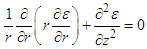 | (26) |
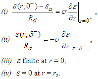 With the rest of the present section emphasizing [10], conditions (iii) and (iv) are imposed to have a solution of equation (24) is in the form
 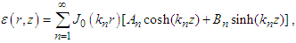 | (27) |
 Applying boundary conditions (i) and (ii) gives
 and
and 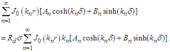 The coefficients An and Bn by multiplying both sides of the above two equations by rJ0(kmr), integrating with respect to r over [0,r0] and applying the orthogonality property of the Bessel functions. Substitute the resulting expressions into equation (25) and get
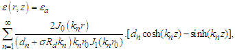 | (28) |
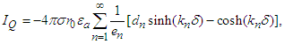
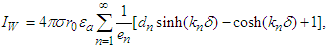
 The gap region accommodates current density
  with
with  given by equation (28) above. Three notable currents come to play. They are the currents crossing the active and quiescent disc surfaces and the current across the cylindrical wall at r = r0 (0 < z < δ). Denote these currents by IA, IQ, and IW respectively. The total current flowing into the gap from IA is
 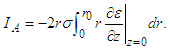 The current flowing into the quiescent cell is
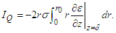 The residual current, IW, across the cylindrical gap boundary is
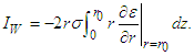 Substitute equation (26) into the above three equations and interchange the order of integration to get
 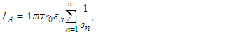 | (29) |
 | (30) |
 | (31) |
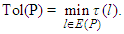
3.3. Source-Sink Analysis
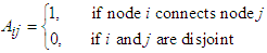
- Source-sink interaction, which is achieved through excitation, is a sine qua non to the proper functioning of the SAN and other cardiac cells. The excitability of a cell can be expressed loosely as the ease with which a response could be prompted. It is often described as the least possible current necessary to depolarize the membrane to the threshold potential [31]. Electric sources of bioelectric origin are generated by the passage of current across the membrane of active (excitable) cells. How depolarizing ‘source’ current generated by the SAN drives depolarization and activation of the contiguous atrial tissue (current ‘sink’) remains uncertain. Bioelectric sources can refer to surface/volume distributions of two types of source elements, that is, the monopole and/or dipole. The dipole is a combination of a source and sink of equal strength. In the conduction system, the self-excitatory SAN is the leading source of action potential. (Note: From Fig. 1(b) or using (17) we have)
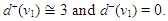 The zero indegree indicates the inherent self-excitatory property Of the SAN. The SAN and the AVN constitute a dipole. In a similar mode, the AVN and the HIS bundle constitute a dipole. In effect, every activated sink becomes a source. Suppose f is a feasible flow and [S, T] is a source/sink cut, then the net flow out of S and net flow into T equal val(f). Assume flow from SAN to HIS bundle is feasible (as in a physiological flow), we have
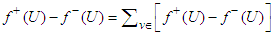 | (32) |
 . Thus, the potential of a unit source located at some point
  inside the tube, which is bounded above and below by the planes z = −L and z = L and on the sides by the cylinder
  = a may be sought. As L approaches infinity the field of the point source inside the conducting cylinder is given by [32]
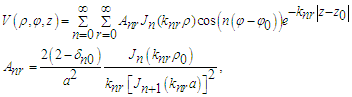 | (33) |
 | (34) |
 | (35) |
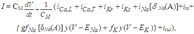
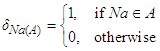
 Na+ is the sodium ion;ist is the sustained current;ito is the transient outward current.Cm is the membrane capacitance.The canonical form of the equation of transmembrane current is (23)
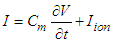 Considering equations (29) and (23) and taking the SAN as the active cell (source), the transiting current, which would drive depolarization and activation of the contiguous cell is
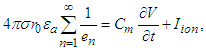 | (36) |
 | (37) |
 | (38) |
3.4. Node-Edge Capacity and Maximal Flow
- A source-sink mismatch is a deleterious liability to numerous impulsive systems. Some biological systems manage to overcome source-sink imbroglio through some anatomical topology. Bartos et al. [34] noted that the ability of SAN to overcome the source-sink mismatch to activate the surrounding atrial myocardium stem from the distinctive anatomy of gap junction proteins. The capacity of an edge cij may be expressed as the bandwidth of the edge, being the maximum flux that the edge can deliver devoid of cramming or damage. Thus, the capacity bandwidth of an edge is inversely proportional to the edge resistance, we write
 | (39) |
 | (40) |
 | (41) |
 | (42) |
 | (43) |
 | (44) |
 | (45) |
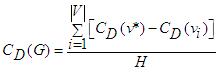
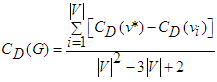
3.4.1. AVCS Global Efficiency
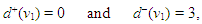
- The question of AVCS global efficiency may be difficult to furnish from the standard equation (6). This arises from the fact that for each of the expressed nodes vk, other than the SAN, d−(vk) = 1. It is of note that, by Definition 2, the AVCS graph is not strongly connected.The centrality concept measures the importance of nodes in a graph network. Here the graph is the GAVCS whose nodes are not interconnected. Centrality may be from the standpoint of the impact of a node on other nodes. Following [37], let v* be the node with the highest degree centrality in G. Let
 be the |Y| node connected graph that maximizes the quantity (with y* being the node with highest degree centrality in X):
 | (46) |
 | (47) |
 | (48) |
 AVN:
AVN: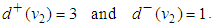 | (49) |
 | (50) |
 | (51) |
4. Summary and Conclusions
- Sources and sinks are typical of flow phenomena. A source is a place/point of inception of flow whereas a sink is a place/point of accumulation of flow. Thus, a sink is a negative source. In nature, there is no presupposition of all-time source and sink of equal strength (dipole). In the bioelectric flow considered, sources and sink mismatch exist without prejudice to the physiological vivacity of the immediate and remote cells involved in the mechanism of flow. The bioelectric conductor considered here is the AVCS. As a rule, the driver of cell-to-cell AP is ionic current. Although the heart is both functionally and anatomically complex, humans, and perhaps animated life with cardiac structures, are compensated by the non-strongly connected nature of its electric flow network. A strongly connected network system is more or less a culprit in the event of deleterious cascading failures. In the event of SAN failure, the AVN is a known surrogate pacemaker, which can initiate the firing of AP to the contiguous cell, the His bundle. In the absence of autonomic nervous stimulation, the rate of ventricular contraction is set at 40–60 bpm by the AVN. It is instructive to note that the serial surrogate responsibility of the AVCS cells is largely compensatory and as well averting. Source and sink system is a network issue. This work employed the benefits of graph theory in analyzing the AVCS. An essential requirement of a network is the efficiency of the edge and nodal structures. Global efficiency is a measure of cumulative effect of the edge-nodal system, especially concerning strongly a connected weighted graph. Given the nature of connectedness of the AVCS, cardiac efficiency is often defined in terms of the mechanics of the heart rather than the electrical system (see for instance [39]). Some interesting points are worthy of note/ emphasis: (i). The AVCS consists of pairs of sources and sinks of unequal strength.(ii). Source and sink mismatch of the AVCS is anatomical, but it may be implicated in pathophysiological conditions. (However, in an anatomical state, it would not be an independent marker of a cardiac event.) (iii). The non-strongly connected nature of the AVCS is an ethereal blessing, as it slows down the rate of cascading failures following any segmental/nodal disorder. This accounts for the relative enduring life of the critical organs in the event of mild to serious AVCS disorder. (iv). The cost of achieving maximal flow is not of necessity an economic one; it requires maintaining the node-edge vivacity. Since autochthonous electrical excitation resides in the SAN, which is the source of AP transmission, and since the other conduction nodes are surrogate pace-makers, it is reasonable to believe that the resolution of conduction anomaly can be found by in-depth analysis of source and sink system associated with the AVCS.
ACKNOWLEDGEMENTS
- The authors are grateful to the reviewers for their meaningful input that helped in the revision of this work.