Abonongo John, Ida Anuwoje L. Abonongo
School of Mathematical Sciences, Department of Statistics, C. K. Tedam University of Technology and Applied Sciences, Navrongo, Ghana
Correspondence to: Abonongo John, School of Mathematical Sciences, Department of Statistics, C. K. Tedam University of Technology and Applied Sciences, Navrongo, Ghana.
| Email: |  |
Copyright © 2021 The Author(s). Published by Scientific & Academic Publishing.
This work is licensed under the Creative Commons Attribution International License (CC BY).
http://creativecommons.org/licenses/by/4.0/

Abstract
Loss reserving for non-life insurance involves forecasting future payments due to claims. Accurately estimating these payments are vital for players in the insurance industry. This paper examines the applicability of the Mack Chain Ladder and its related bootstrap predictions to real non-life insurance claims in the case of auto-insurance claims from Bolgatanga State Insurance Company branch. The results showed that, the mean IBNR and Ultimate reserves from the bootstrap technique produced results that are close to that in the Mack model. The prediction errors from the bootstrap technique are higher than that of the Mack model. It was realized that, the cdf of the IBNR claims follow a log-normal distribution; this distribution was fitted from the bootstrapping with 999 replications. Also, 75%, 90%, 95% and 99.5% were the quantiles used in measuring the IBNR VaR and it was realized that 2016 recorded the highest IBNR VaR. The prediction errors from the bootstrap technique are higher than that of the Mack model. It was realized that, the cdf of the IBNR claims follow a log-normal distribution. This distribution was fitted with mean of 14.030 and standard deviation of 0.293 from bootstrapping with 999 replications. Also, the accident year (2016) recorded the highest VaR estimates.
Keywords:
Claim reserves, Mack Chain Ladder, Bootstrapping, Accident year, Development year, IBNR claims
Cite this paper: Abonongo John, Ida Anuwoje L. Abonongo, Loss Reserving -the Mack Method and Associated Bootstrap Predictions, Applied Mathematics, Vol. 11 No. 3, 2021, pp. 29-36. doi: 10.5923/j.am.20211103.01.
1. Introduction
Mostly, revenue of insurance companies are based on the premiums collected, while the expenses arise from having to compensate the insureds. Thus, companies at least need to gather premiums that can cover for future losses. At the time of gathering premiums, the losses arising from the collective of individuals are unknown. Therefore, the sizes of individual premiums must reflect the future distribution of losses, derived from separate uncertainties. The severity of future loss is reflected by individual risk characteristics as well as frequency (the number of individuals who are covered).An individual who has purchased an insurance policy can file for compensation, in the event of accident. Such a request of compensation arriving at an insurance company is referred to as a claim.Reserving in the insurance business is the process of setting aside capital to cover the losses for claims that have occurred in the historical accident periods. At a certain stopping time t, the premiums collected must cover the liabilities (both paid and outstanding) originated from before that point in time (Norberg (1993)). Some parts of the liability at time t might include payments that are made in the future, however, insurance companies are not allowed to forecast future premiums to cover those outstanding liabilities. Thus, reserving in insurance comes down to making estimations and predictions of the unknown future development of claims that have occurred during the current or previous accident years. This involves predicting development of reported but not settled claims as well as IBNR (Incurred But Not Reported) claims.In recent years, bootstrapping has become famous in loss reserving. Also, it is upfront to use it to obtain the approximation to the prediction error and the predictive distribution of a statistical process by including simulations from underlying distributions. Therefore, making it a powerful tool for loss reserving purposes in non-life insurance, the prediction error of the reserve estimates. It should be noted that, to obtain the predictive distribution, rather than just the estimation error, it is essential to use the bootstrap procedure by simulating the process error.One of the major challenge in every day actuarial practice is selecting the loss development factors. The adjustments to make data more homogeneous are often justified for number of reasons: unstable run-off-triangles, outliers, inaccurate and incomplete data, among others. Most actuaries use picking up rules of thumb and helpful approaches in selecting the loss development factors (LDFs).Duval and Pigeon (2019), proposed models for non-life loss reserving by combining traditional approaches such as Mack’s or generalized linear models and gradient boosting algorithm in an individual framework. Their models used information about each of the payments made for each of the claims in the portfolio, as well as characteristics of the insured. Also, they models provided a contrast for some traditional aggregate techniques, at the portfolio level, with their individual-level approach.Some contributions on loss reserve estimate are focus on the strengths and weaknesses of several evaluation models used. Most of the research are on nominal no discount value of loss reserve in line with constitutional reserve obligation. Traditionally, some of the methods are based on historical inflation to give the nominal reserves. Outstanding losses are faced with inflation till they are paid; if inflation rate during the period is high, loss severity will increase, leading to large loss reserves. Also, when inflation rate is low, then the loss severity during the period will increase, leading to a lower loss reserves.The most commonly used method in loss reserving is the chain ladder method. The chain ladder method is a distribution-free method, relieving some of the usual assumptions common to most modeling techniques. This method is used by formulating a common ratio of losses between subsequent development years (Mack (1993)). The assumption of the chain ladder method is that subsequent claim years are independent (Wuthrich and Merz (2008)). Some variations on the basic chain ladder method (Gerhard and Mack (2004)) can also be used to estimate other values such as reserves and current excess reserves, as well as estimating the standard error of these predictions (Schnieper (1991)). Calculating the standard error of the chain ladder method and quantifying the uncertainty with these different variations in the chain ladder method is a helpful way of evaluating the differences between the various methods (Mack (1993)).The distribution-free chain ladder method has underlying models that have been the subject of more recent research. These newer models assume claim amounts follow a specific distribution and can lead to the same estimates as the distribution-free chain ladder method. For example, a Poisson model for claim counts can lead to the same expected number of claims as the distribution- free chain ladder estimates (Wuthrich and Merz (2008)). Generalized linear models (GLM) have been historically popular in the field of loss reserving, and the increased access to user-friendly statistical software has further bolstered the popularity of methods using GLM (Haberman and Renshaw (1996)). Extended Link Ratio techniques, including weighted least squares regression, have been shown to be effective in handling various insurance lines of loss triangle data (Barnett and Zehnwirth (2000)).England and Verrall (2002) published a report presenting various stochastic techniques for loss reserving that had been developed at that time. The authors presented a number of aggregated models such as extensions of Chain-Ladder or Bornhutter-Ferguson, where cumulative or incremental payments for portfolio accident years were considered. Also, some micro-focused approaches were discussed where number of claims for a period was modelled by a Poisson distribution, similar to the approach presented in Norberg (1993).Norberg (1986) published a paper tackling the issue of predicting IBNR-claims (Incurred but not reported). He used a wide framework and various specifications of model as assumptions. As data was grouped annually, basic model assumptions included yearly risk measures of exposure as a known quantity. Each year was paired with quantities representing the latent general risk conditions which were assumed to be unobservable random elements. The total amount of claims occurring during an accident year was assumed to be Poisson distributed.Mack (1993) published an article on the prediction error of the Chain Ladder method.The research answered the question of actual variations to the other models and also measured the differences in actual reserves for insurers. Also, it was revealed that, the new developed model exhibited an important view on how to estimate the parameters for Bornhuetter Ferguson (B-F) claims reserve method. The stochastic model identified what was meant by initial estimate for the ultimate claim reserves. In using the formula for prediction error, Mack's research urged actuaries to access their doubt on the sets of parameter, the development pattern and initial claims amount.Moreover, Schmidt (2006) also published an article on some methods for modeling claims which made use run-off triangle. The research revealed that, under the assumption that the development of losses of each accident year follows a development pattern which is common to all accident year then, the use of the run off triangle could be accepted. This theory was viewed as a primitive stochastic model of claim reserving. He also realized that, a development pattern become a unifying force in the comparison of the models which to a great extent could be under the B-F method. The additive method, loss development method, Cape-Cod method and Chain ladder methods could be seen as unique cases of the actual B-F method. The paper further corrected these methods by statistical inference used on sophisticated and suitable stochastic models in that, Gauss-Markov and credibility predictions as well as maximum likelihood estimation can contribute significantly to the understanding of various methods of loss reserving.Furthermore, Mack (1993) published an article on the chain-ladder estimates and ways to calculate the variance of the estimate. Murphy (1994) also offered other variations of the chain-ladder method in a regression setting.The purpose of this paper is to simply show the applicability of the Mack model and its associated bootstrap predictions to real non-life insurance claims in forecasting/ estimating IBNR (Incurred But Not Reported) claims. Also, this paper adds to literature as to applicability of the bootstrapping technique in fitting non-life insurance claims especially with regards to the underlying distribution of the claim amounts.
2. Materials and Methods of Analysis
2.1. Source of Data
Secondary data on motor insurance paid claims from SIC Bolgatanga branch spanning from 2012 to 2016 was employed.
2.2. Methodology
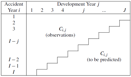
2.2.1. Run off Triangle
If  denote the random variables (incremental payments, cumulative payments) for accident year
 until development year
  where the accident year in which an event causing a loss occurs. Assume that
  are random variables observable for calendar years
  and non-observable for calendar years
  . The observation
  are represented by the so called run off trapezoids
  or run off triangle
2.2.2. Outstanding Reserves
Let  denote the outstanding claims liabilities for accident year
  which is given
 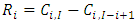 | (1) |
and  denote the total outstanding loss liabilities for accident years given by
  | (2) |
Let  and
and  denote the claims reserves for accident year
 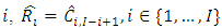 and the total claim reserves for aggregated accident years,
  respectively, where
  is predictor for
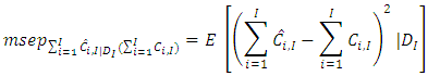
2.2.3. Conditional Mean Square Error of Prediction (MSEP)
In finding a suitable prediction of ultimate loss, the insurer need to assess the variability of these loss amounts. Thus, one is interested in quantifying the prediction uncertainty of the ultimate loss i.e,  and
and  , equivalent of claims reserve, i.e,
  and
and  . Then, choosing an appropriate risk measure which determines a conception of measuring the distance between the prediction and the actual outcomes. Hence, the MSEP is given by
 | (3) |
 | (4) |
where  .
.
2.2.4. Mack Chain-Ladder Method
A method which estimates the standard error of the chain-ladder forecast without as- suming distribution was published by Mack (1993). Thus, the Mack Chain-Ladder model estimates/forecasts future claims development based on a historic cumulative claims development triangle and estimates their standard errors. The Model Assumptions of Mack Chain-Ladder Method are as follows:Defining the individual development factors, for 
 and
and 
 | (5) |
CL1: There exist constants  such that
 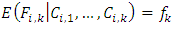 , where
  is the loss development factor (LDF), link ratio or age-to-age factor.CL2: There exist constants
  such that for all
  and
and  . Then,
  with
with  , where
  is the variance parameter. CL3: The accident years
  are independent. If these assumptions hold, the Mack Chain Ladder gives an unbiased estimator for IBNR (Incurred But Not Reported).
2.2.4.1. Estimating the Parameter in the Mack Chain-Ladder Model
Given the information  and for
  , the development factor or age-to-age factor are estimated by
 | (6) |
where  is the weight,
  is the individual development factor,
  is the future loss
  is the previous loss.Also, given the information
  and for
 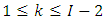 , the variance parameter is given by
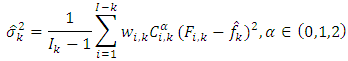 | (7) |
2.2.4.2. Properties of the Estimators from Mack Chain Ladder Model
1. The estimators  are unbiased and uncorrelated.2. The estimator
  for
for  have the minimum variance among all unbiased estimators of
  which are the weighted average of the observed development factors
  3. The estimator
  is the unbiased estimator of the parameter
  .4. Under property 1 and 3,
  meaning, together with the fact that
  are uncorrelated, that
  is unbiased estimator of
  .5. The expected values of the estimator,
 for the ultimate claims amount and the time ultimate claims amount
  are equal i.e
2.2.4.3. Estimators of the Conditional MSEP in Mack Chain-Ladder Model
For single accident years, the assumptions of Mack Chain-Ladder model have the following estimator for the conditional estimation error, 
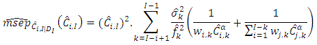 | (8) |
where for 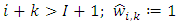 and
and  and
and  are as defined earlier. Also, for aggregate accident years, the MSEP is given by
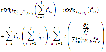 | (9) |
2.2.5. Bootstrapping the Chain Ladder
The following algorithms are involved in bootstrapping the chain ladderi. Estimate development factors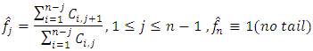 | (10) |
ii. Fit chain ladder to the original data and predict bottom-right triangle | (11) |
iii. Back-fit observed original claims from diagonals 
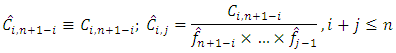 | (12) |
iv. Calculate un-scaled Pearson residuals 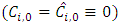
 | (13) |
v. Resample residuals  B-times with replacement. Thus, B triangle of bootstrapped residuals
  vi. Construct B incremental bootstrap triangles
 | (14) |
vii. B cumulative bootstrap triangles 
 | (15) |
viii. Perform chain ladder on each bootstrap cumulative triangle. Thus, reserves  Therefore, (v) to (viii) is a bootstrap loop (repeated B-times)ix. Empirical distribution of size B for the reserves. Thus, empirical (estimated) mean, standard error, quantiles among others are obtained.
3. Application to Data
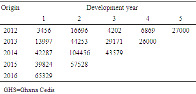
Table 1 shows the incremental paid claims data as a run off triangle. The rows represent all claims relating to accidents that occurred during a given year (origin). The columns represent the development years (dev) which indicates how the cohort of claims relating to a particular accident year evolve over time. The development year (dev) for a claim settlement reflects the time taken after the amount was settled. Thus, the amount of loss that occurred in an accident year (origin) is considered settled in dev 1, the amount of loss settled in the following year is in dev 2 and so on. This means that, for accident year (origin) 2012, 2013, 2014, 2015 and 2016 in dev 1, 2, 3, 4 and 5; 3456, 16696, 4202, 6869 and 27000 claims were settled respectively. The diagonal claims paid represent the claims amount settled in a single calendar year (origin). For instance, the last diagonal (from dev 1 to dev 5) containing the following settled claims; 65329, 57528, 43579, 26000 and 27000 includes all payments made during the most recent calendar year (2016). It could be seen that, the lower right corner of Table 1 has no payment amounts and thus represents the time period in the future for which there is the need to estimate the expected loss amounts ie. IBNR claims.Table 1. Incremental claims (GHS'000)
 |
| |
|
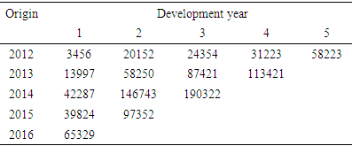
The cumulative claims paid is shown in Table 2. It is the sum of all loss paid up to that development year. Thus, claims in the last diagonal (65329, 97352, 190322, 113421 and 58224) equal the sum of the paid claims to date for each accident year (2012, 2013, 2014, 2015 and 2016) respectively.Table 2. Cumulative claims (GHS'000)
 |
| |
|
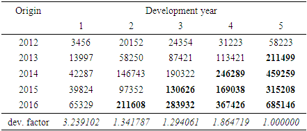
Table 3 shows the Mack full triangle of the loss settled and to be settled (IBNR claims).Table 3. Mack Full triangle (GHS'000)
 |
| |
|
In estimating the outstanding loss reserves (IBNR claims), the cumulative paid claims in Table 2 is used. This is done by simply completing the lower right triangle. Thus, by multiplying the development factors with the last observed claim in each accident year and development year. The process continues until the triangle is complete. For instance, in the last accident year (2016) the IBNR claims; 211608, 283932, 367426 and 685146 were obtained by multiplying 65329 by 3.239102, 211608 by 1.341787, 283932 by 1.294061, 367426 by 1.864719 respectively. This same technique is applied to the rest of the accident years (origin) to obtain the IBNR claims. Also, the 211499 claim exhibited in origin 2013 in dev 5 is the IBNR claim for the accident year (origin) 2017. For accident year 2014, the 246289 and 459259 in dev 4 and 5 respectively are the IBNR claims for 2017 and 2018. The IBNR claims (130626, 169038 and 315208) for 2015 in dev 3, 4 and 5 are for the accident year 2017, 2018 and 2019 respectively. For the accident year (2016), the 211608, 283932, 367426 and 685146 are the IBNR claims for the accident year 2017, 2018, 2019 and 2020 respectively.Figure 1 shows the diagnostics plot of the chain ladder in verifying the Mack assumptions. It could be seen that, there are no trends in the four residual plots and for that matter the Mack assumption holds. The Chain ladder development by origin period exhibits similar trend for dev 1 to 5. Also, from the origin period and forecast amount in the first figure from the left, it could be seen that, there is no forecast region for the origin (2012) because the development years are fully developed. In 2013, only one claim amount (small severity) was forecast giving rise to smaller forecast region followed by 2014 and 2015 with two and three forecast claims respectively with fair forecast regions but the forecast claims size for 2014 is bigger than that of 2015 and thus, the forecast region of 2014 wider than 2015. Since the accident year 2016, had four (highest) predicted claims, it had the highest forecast region.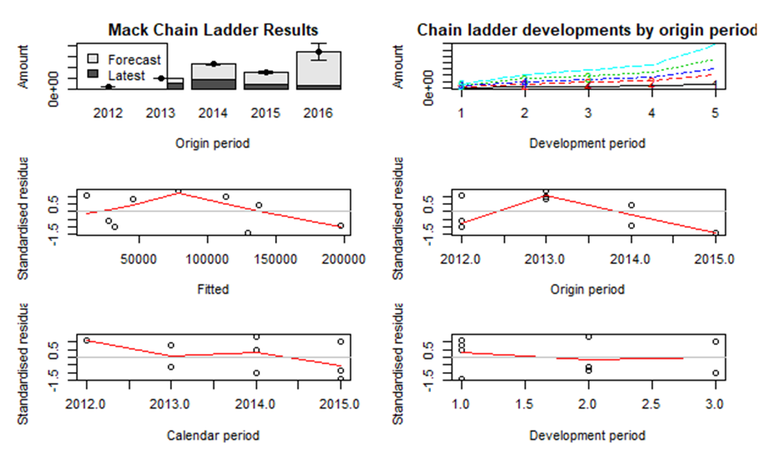 | Figure 1. Chain Ladder Diagnostics |
Figure 2 shows the plot for the chain ladder with Mack's standard error. Each plot shows one occurrence year (origin) ie. 2012, 2013, 2014 and 2015. It also shows the evolution of the cumulative amounts paid over time. The solid lines represent the evolution cumulative payments for future periods which are unobserved whereas the dash lines show a plus one or minus one standard error as obtained from Mack approach. Therefore, the evolution of the cumulative amounts paid are very low in 2012 and 2013, meaning the claims paid incrementally were not much compared to the amount paid in 2014, 2015 and 2016. The claim amount paid in 2015 is higher meaning much claims got evolved than that in 2014 and 2016. Also, the standard error for 2012, 2013 and 2014 are not observed compared to 2015 and 2016 which are clearly observed an indication of high standard error.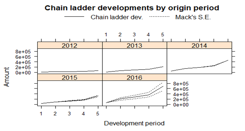 | Figure 2. Plot of chain ladder with Mack's standard error |
Figure 3 shows the plot of Mack full triangle. From the plot it is observed that, the paid claims for the fully developed triangle follows the same trend. This means that, the data is stable and is not much spread out. There is also not much difference in the claims paid previously compared IBNR claims.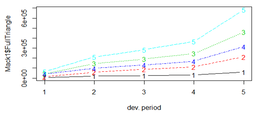 | Figure 3. Plot of Mack Full triangle |
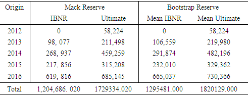
Table 4 shows the reserves for Mack model and bootstrapping. It could be seen that, the Mack IBNR reserve and the mean IBNR of the bootstrap distribution are close to each other. Also, there is no significant difference between the Ultimate reserve for the Mack model and the mean Ultimate reserve from the bootstrap technique. This means that, the bootstrap technique is able to produce claims similar to that of the Mack model.Table 4. Mack and Bootstrap Reserves
 |
| |
|
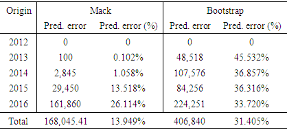
Therefore, the bootstrap mean IBNR and ultimate reserve, could be used to make further inference.Table 5 shows the Mack and bootstrap prediction error. It is realized that, for the Mack Model, the highest prediction error is recorded in 2016 (26.114%) and the least prediction error in 2012. This is because in 2012 (0), the development years were completely developed and thus no IBNR claims were estimated whereas 2016 had the highest IBNR claims estimated. The prediction error in the bootstrapping had 2013 (45.532%) exhibiting the highest prediction error with 2012 (0) exhibiting the least prediction error.Table 5. Mack and Bootstrap Prediction Errors
 |
| |
|
After employing the bootstrapping technique (simulation) with 999 replication, the plots in Figure 4 were obtained. It can be realized that, the is not much difference between the latest actual incremental claims and simulated values. The graph for the cdf of the total IBNR tends to follow a log-normal distribution. This is also depicted in the histogram of the total IBNR.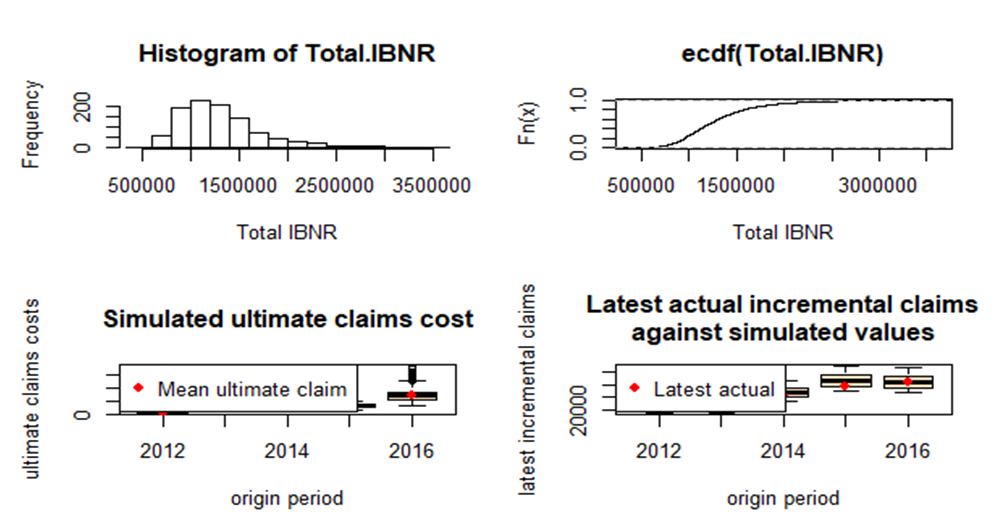 | Figure 4. Bootstrap Results |
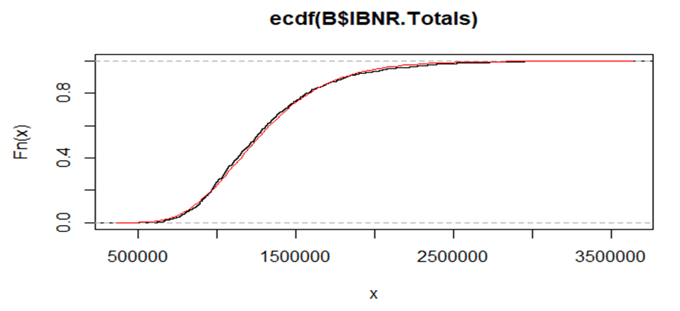 | Figure 5. Fitted log-normal distribution |
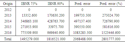
Since the cdf of the total IBNR tends to follow the log-normal distribution, there is the need to fit it. This was done with mean of 14.030 and standard deviation of 0.293. The fitted distribution is illustrated by the red line.Table 6 shows the bootstrap IBNR quantiles at 75%, 90%, 95% and 99.5%. These are measures for VaR. It can be seen that the accident year (2012) exhibited 0 for the four quantile estimates. This is because 2012 is fully developed in terms of paid claims and that there are no IBNR claims. All the four quantiles had 2016 recording the highest VaR value of 775509.900, 969640.900, 1083283.500 and 1523446.600 for IBNR at 75%, 90%, 95% and 99.5% respectively.Table 6. Bootstrap IBNR Quantiles
 |
| |
|
4. Conclusions
Claims reserving forms an integral part of non-life insurance operations. The purpose of this paper is to illustrate the applicability of Mack Chain Ladder and its bootstrap predictions on real non-life insurance data in estimating or forecasting reserves. But since the Mack Chain Ladder is a distribution free chain ladder method, the bootstrap technique was applied in fitting the underlying distribution of the reserves. The results showed that, the mean IBNR and Ultimate reserves from the bootstrap technique produced results that are close to that in the Mack model. The prediction errors from the bootstrap technique are higher than that of the Mack model. It was realized that, the cdf of the IBNR claims follow a log-normal distribution; this distribution was fitted from the bootstrapping with 999 replications. Also, 75%, 90%, 95% and 99.5% were the quantiles used in measuring the IBNR VaR and it was realized that 2016 recorded the highest IBNR VaR. Therefore, in applying a distribution free chain ladder model, it is prudent to ascertain the underlying distribution of the reserves so as to make good inference about the IBNR reserves. This is because the moment characteristics (mean, standard error, etc) of the Mack model does not provide full information about the reserve distribution and that the mean and variance alone do not contain full information on the distribution (cannot provide the VaR). From Norberg (1986), this paper also predicted IBNR-claims using the bootstrapping technique; it helped in fitting the claim amounts to a statistical distribution.
Conflict of Interest
The author declare that there are no conflicts of interest regarding the publication of the article.
ACKNOWLEDGEMENTS
We wish to acknowledge SIC Bolgatanga branch for the data.
Funding
This work was done as part of our employment; C. K. Tedam University of Technology and Applied Sciences, Navrongo.
References
| [1] | Barnett, G. and Zehnwirth, B. (2000). Best estimaes for reserves. Proceedings of the Casualty Actuarial Society, LXXXVII: 245-321. |
| [2] | Duval Francis and Pigeon Mathieu (2019). Individual loss reserving using a gradient boosting-based approach. Risks, 2019, 7, 79. |
| [3] | England, P. D. and Verrall, R. J. (2002). Stochastic claim reserving in general insurance. British Actuarial Journal, 8(3): 443-518. |
| [4] | Gerhard, Q. and Mack, T. (2004). Munich chain ladder. Blatter Der DGVFM, 26(4): Springer: 597-630. |
| [5] | Haberman, S. and Renshaw, A. E. (1996). Generalized linear models and actuarial science. Journal of the Royal Statistical Society D (The Statistician), 45(4): 407-436. |
| [6] | Mack, T. (1993). Distribution-free calculation of the standard error of chain ladder reserves estimates. ASTIN Bulletin. The Journal of the IAA, 23(2): 213-225. |
| [7] | Murphy, D. (1994). Unbiased loss development factors. PCAS, 81:154-222. |
| [8] | Norberg, R. (1986). A contribution to modelling of ibnr-claims. Scnadinavian Actuarial Journal, (3-4): 155-203. |
| [9] | Norberg, R. (1993). Prediction of oustanding liabilities in non-life insurance. ASTIN Bulletin, page 1: 95115. |
| [10] | Schmidt, D. K. (2006). Optimal and additive loss reserving for dependent lines of business. CAS, Call for paper program. |
| [11] | Schnieper, R. (1991). Separating true ibnr claims and ibnr claims. ASTIN Bulletin, 21. |
| [12] | Wuthrich, M. and Merz, M. (2008). Stochastic claims reserving methods in insurance. John Wiley and Sons Ltd, New York. |

 Abstract
 Reference
 Full-Text PDF
 Full-text HTML