1. Introduction

1.1. Background of the Study

Life is said to be full of uncertainties and risks; expected and unexpected, certain and uncertain. Recently there has been a lot of losses due to unfortunate happens that are out of control of owners all over the globe affecting personal lives and the business environment. Particularly in Ghana, many adverse events such as occupational hazards, theft and burglary, traffic and motor accidents, fire outbreaks and accidental damage to property and harm caused to lives as well as unknown events have negatively affected the activities of the private sector especially that of SMEs. These uncertainties and mishaps remind of the fact that there is a need to undertake risk management measures to save guard the business. The possibility that these adverse events will occur creates a risk to the entrepreneurs of the business, which through insurance contracts transfers to insurance companies so that now on the side of the insurance companies, there is also a risk to lessen the burden of loss when these events occur. Risk is everywhere and whether it is evitable or not the business world is very much exposed to it especially with the private sector where businesses are many owned by individuals and private corporations. To overcome the losses arising from these risks, some businesses undertake insurance covers unfortunately others do not. The uncertainty about business management and decisions in the future and the resulting gains cannot be optimistic (Aizeman and Marion, 1999). The response of the sector despite many efforts by successive governments through workshops, seminars and reforms to improve the sector and compliment government investments have not been encouraging in the past years and the problem could be because of the risk adverse behaviour of owners. It is true that venturing into risky ventures yield returns on investment but there is also a need for a backup plan and that in view of this is an investment plan or cover so that in case of any mishaps there is always a recovery plan. The patronage of insurance as a risk management tool provides that confidence in business decisions, however to some degree and extent. The basic function of insurance is the transfer of risk. According to the California insurance code, section 22, insurance is a “contract whereby one undertakes to indemnify another against loss, damage, liability arising from a contingent or unknown event”, to indemnify a person is to transfer a risk from one party (the insured) to another (the insurer). This transfer of risk doesn’t necessarily remove or take away the possibility of a loss, damage or liability arising from a contingent or unknown event, rather the insurance to an extent takes upon himself to provide some sort of financial security or compensates with something of monetary value to cover for the misfortunes hitting the insured with the insured with the insured risk occurs. In return, an insured pay a premium in a very small amount usually called a money consideration when compared with potential losses that may be suffered as a result. Insurance in Ghana as risk management tool was made compulsory by the Insurance Act, 2006 (Act 724), where it was made compulsory for every owner to obtain fire and liability insurance cover. Sections 183 and 184 of the Act stated that, “a person shall not construct or cause to be constructed a commercial building without insuring with a registered insurer the liability in respect of construction risks caused by negligence or the negligence of servants, agents or consultants which may result in bodily injury or loss of life to or damage to property of any workman on the site or of any member of the public; every commercial building shall be insured with an insurer against the hazards of collapse, fire, earthquake, storm and flood, and an insurance policy issued for it; the insurance policy shall cover the legal liabilities of an owner or occupier of premises in respect of loss of or damage to property, bodily injury or death suffered by any user of the premises and third parties”. Unfortunately, this Act has not been heeded to by owners of property and when the inevitable strikes these individuals became victims of circumstance with no help. The recent fire outbreaks in most parts of the country are no exceptions, where many business where lost due to the fires are evidence the need for businesses to take insurance covers to minimise the effects of hazards to SMEs, Government agencies and departments; calling on stakeholders and the government to assist victims.

1.2. Problem Statement

SMEs in Ghana are noted as the bedrock of the emerging private sector and serve as sources of growth, technological innovation and flexibility. Representing more than 90% of all businesses in Ghana, SMEs are unfortunately exposed to many risks in the line of business. In spite of this risk is overlooked by SMEs despite the fact that operating a business comes with a lot of risks that are inevitable. However, prudent business owners knowing well that risk is inevitable take steps to minimize their risk thereby maximising returns of investment. However the Insurance Act 724, Section 183 and 184 is unfortunately not heeded to despite the fact of its significance to reduce the effects of risks resulting from uncertainties that spring up in the course of business. Therefore the question now is after the loss is suffered when the events occur, do these SMEs or businesses have a recovery measures or measures to get back on their feet? This study seeks to examine the patronage of SMEs in non-life insurance policies as a risk management tool laying emphasis on the Kumasi Metropolitan Area and also determine whether a business owner would opt for an insurance cover to minimize such losses?

1.3. Objectives of the Study

The study intends to achieve the following objectives:

1. Determine whether a business owner would opt for an insurance cover to minimize such losses?

2. To predict the likelihood for an individual to go in for insurance covers.

3. To determine or check the performance of the model.

4. Find out solutions to these problems.

1.4. Significance of the Study

The study would help identify the reasons for the level of patronage of insurance as a risk management tool and create a changed behaviour of the owners of SMEs. Also it would aid risk managers of insurance companies would preparing risk management policies especially in the area of SMEs.

1.5. Organisation of the Research

The study is divided into five (5) chapters. Following from above, chapter two of the study concentrates on reviewing literature on SMEs and Insurance as a risk management tool. Chapter three involves the research methodology. Chapter four involves the presentation, analysis and interpretation of data collected in the study collected on the topic. The last chapter presents findings, conclusions and recommendations.

2. Definition of SMEs; Overview and Key Definition

SME basically stands for Small to Medium Enterprise. However, what exactly an SME is depends on who is doing the defining. There is no universal definition to define SMEs. Small and medium-sized enterprises (SMEs) are non-subsidiary, independent firms which employ less than a given number of employees. This number, however, varies across countries, (William, 2000; Bakare, 2009). Industry Canada uses the term SME to refer to businesses with fewer than five hundred (500) employees, while classifying firms with 500 or more employees as large businesses. In trying to further define SMEs, Industry Canada defines a small business as one that has fewer than one hundred (100) employees (if the business is a goods-producing business) or fewer than fifty(50) employees (if the business is a service-based business). A firm that has more employees than the cut-offs but fewer than 500 employees is classified as small to medium enterprises. In its on-going research program that collects data on SMEs in Canada, Statistics Canada defines SMEs as one with 0 to 499 employees and less than $50 million in gross revenues (Susan Ward, 2013). Different countries across the world define SMEs in different ways, based on number of employees and turnovers from the business. In the European Union (EU), a similar system is used to define SMEs. A business with a headcount of fewer than two hundred and fifty(250) is classified as Medium sized, a business with a headcount of fewer than fifty(50) is classified as Small ,and that of ten (10) a micro business. The EU system also takes account of a business turnover rate and its balance sheet. Many researchers all over the world have battled with the relevant criteria for defining SMEs. This could arise from two sides:

1. Industrial and economic differences across sectors and countries around the world. Per the industrialisation and the economic growth of one country, its definition of what a SME is would differ from another country, also, in the difference in the sectors would also because the definitions to differ, a small firm in the oil industry might probably have much higher levels of capitalization than a small firm in the service sector.

2. Economic aggregates used to base the analysis could be a factor influencing the settlement on the definition for SMEs, hence the classification of SME according to employees, turnover, profitably or net worth. (Potobsky, 1992). Various attempts to overcome this definition problem have been made without much success. Some models classify firms as small if they met criteria of market share, management and level of independence. While other models based their classifications on various sectors of an economy from which an SME might have emerged. In almost all senses, Storey (1994) argued that the EC definitions were more appropriate. A key problem with the EC definitions of an SME; however, is that for a number of developing countries with their sectorial development it is too “all embracing”. In the case of internally domestic purposes within countries, the SME definition would not be helpful (Tonge, 2001). Following from that, the trend had been for each country to define an SME based on criteria that reflected its own micro and macro-economic characteristic sector performances. According to Tonge (2001), the heterogeneity of the small firms sector meant it was necessary to modify definitions according to the particular sectorial, geographic or other contexts in which the small firms were being considered. Based on this fact, Small to Medium Enterprise (SMEs) were variously defined, but the most commonly used criterion was the number of employees of the enterprise. These classifications then depended on various nations with their specific motives for SMEs under sectorial performances, geographic location and financial exchange regimes of a said country in its foreign exchange market with particular reference to time.

2.1. History of SMEs in Ghana

Representing more than 90% of all businesses in Ghana, SMEs occupy a central part of the Ghanaian economy – they put food on the table of many households in Ghana. They are essentially the drivers of the Ghanaian economy even though some of them are hardly noticed. The contribution of SMEs to income, employment generation and ultimate economic growth is therefore not in doubt. (Shika Acolatse, Business Sense 2012). The economic structure of Ghana is focused on three (3) main areas: public sector reform, financial sector reform and private sector development. The government’s policy towards private sector development aimed at creating a more business- friendly economic and regulatory environment, strengthening property rights, seeking expanded market access for Ghana’s exports, and promoting entrepreneurial skills. (Aduko, 2011). The government efforts to reduce poverty and increase economic growth was channelled through SME development in the country. SMEs are mostly found in the urban and rural areas in the country, and it covers from agriculture and farming activities, health, education, the art and craft industry, textiles and clothing, retail, construction services and financial services. SMEs take up employment of close to 70% of the labour force in Ghana. There is a long history of government initiatives to promote and finance SMEs in Ghana. However, financial constrains remained the major restriction to SME development in the country. Ghana began officially promoting the activities of SMEs in 1969 with the establishment of the Credit Guarantee Scheme by the Bank of Ghana to assist entrepreneurs in obtaining bank credit. That was followed in 1970 by the creation of the Ghana Business Promotion Programme. The objective of these initiatives was to aid financially and also to give technical assistance to newly established and existing SMEs, but their impact was limited. Support of SMEs was intensified in 1990 following the creation of the National Board for Small-Scale Industries (NBSSI). The major financing scheme operated by the NBSSI was a credit line - the Fund for Small and Medium Enterprise Development (FUSMED) – financed by the World Bank’s small and medium enterprise project. The credit facility which was handled by the NBSSI was with the intention of assisting entrepreneurs in procuring scarce but essential raw materials. (African Economic Outlook, 2005).

2.2. Characteristics of SMEs

Businesses around the world and even in Ghana have characteristics that show that the firms running these businesses are likely to be SMEs. Some important characteristics and features of SMEs all over the world and most especially Kumasi, Ghana were the study is focused were observable: they are generally more labour intensive than larger businesses; on the average, they generate more direct job opportunities per unit of invested capital; they are an instrument for the talents, energy and entrepreneurship of individuals who cannot reach their full potential in large organisations; they often thrive by rendering services to a segment of the market which larger businesses do not find attractive; they are a means of entrepreneurial talent and a testing ground for new industries; they create social stability, cause less damage to the physical environment than large factories, stimulate personal savings, increase prosperity in rural areas and enhance the population’s general level of economic involvement. In addition, they are usually price followers, whilst ingenuity, creativity and devotion are typically found in them. They are by nature often credited with the ability to bring about social stability in the poorer communities. This is done by generating more job opportunities. These varied characteristics and features even though important expose SMEs to various levels of business risks that effect the business’s operations in the event of uncertainty.

2.3. Challenges of SMEs

Given the features of SMEs, they are faced with a variety of constraints owing to the difficulty of absorbing large fixed costs, the absence of economies of scale and scope in key factors of production, and the higher unit costs of providing services to smaller firms (Liedholm & Mead, 1987; Liedholm, 1990; Steel & Webster, 1990). There are a lot of constrains that SMEs face among which includes input, finance, labour, equipment and technology, domestic demand, regulatory, legal, managerial and institutional constrains. In the case of insurance, there is an assertion that high premiums, non-payment of claims, underpayment of claims, undue delay of claim settlement and under insurance were some of the difficulties faced by SMEs in the metropolis and that majority of the owners of SMEs were not usually interested in securing insurance cover unless under compulsion from the banks when securing financial facilities.

3. Methodology

3.1. Introduction

This chapter looked at the methodology employed to achieve the objective of this study. Specifically, it focused on the population, sampling, research design, and administration of questionnaire, sample size, sampling procedure, data collection and analysis. It also included qualitative and quantitative research regarding the objectives of the dissertation. Limitations of the research encountered by the researchers in the course of the study have been stated.

This section finally described how field data was made suitable for presentation and analysis and the tools used for data presentation and also describe the study area.

3.2. Data Collection Instrument

The tools that were used for the collection of primary data are the interview schedule and questionnaires were exclusively used to solicit the views of the respondents on the research topic. The study was descriptive, in that it was conducted to determine and describe the variables that affected risk management by SMEs and the related insurance policies to mitigate risk. The survey involved the collection of data using questionnaire and observation. Mainly, this study made use of one research instrument designed specifically for the population targeted and complemented by observation. The data collection instruments were a set of questionnaire as in appendix 2. The questionnaires were administered to owners/managers of SMEs and mangers of insurance companies in the Kumasi Metropolitan Area. The questionnaires were chosen because: they enabled a broader survey of the population, they were less stressful than one on one interview, people were more willing to be truthful because their anonymity was guaranteed, and they were easier to analyze. However, the limitations associated with the technique were that: they did not allow the researchers to interact fairly with respondents. The questionnaires were both self-administered and with the assistance of two other personnel; the researcher had a chance to interact with some of the respondents. They were also limited in the depth to which the researcher was able to probe any particular respondent and did not allow for any digression from the set format (Hofstee, 2006; Fisher, 2004). The questionnaires were however designed to deal with the weaknesses. However, the literate respondents were made to fill the questionnaire by themselves with or without the assistance of the researcher.

3.2.1. Questionnaire

The questionnaires were conducted by the researchers and with the assistance of two other persons to collect data from the owners or managers of SMEs and managers of insurance service providers. The questionnaires were structured as appendix 1. The questionnaire contained sections “A” to “C”.

3.2.2. Pre-testing of the Research Instrument

The questionnaire were pre-tested among a sample of 15 selected respondents to check for glitches in wording of questionnaire, ambiguity of instructions, and to avoid anything that could obstruct the instrument's ability to gather data in an economical and systematic manner for the attainment of the research objectives.

3.3. Population and Sample Size

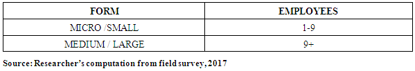
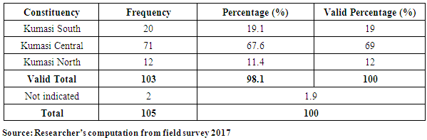
A total of 110 questionnaires were distributed and out of this, 105 were received from the field made up of 90 from entrepreneur, 10 support institutions and 5 from banks. One of the entrepreneurs failed to answer and submit his questionnaire, despite the researcher’s efforts and number of calls made to explain the potential benefits of the study to him, but because of time constrains those received were used for the analysis. Though, there was no registered list of SMEs within the Metropolis with the Registrar General Department; a few lists of registered enterprises were obtained from National Board for Small Scale Industries (NBSSI) and Business Advisory Centre (BAC). The exact population of SMEs in Kumasi Metropolis was unknown. However, 50 Micro/Small Enterprises, 42 Medium Enterprises were sampled. In addition, all the 15 Non-life Insurance companies in the Metropolis formed part of the respondents to determine the level of patronage by SMEs. The total sample size was 110 respondents. This clustering was done because the researcher intended to ensure that all sections of the Metropolis were covered. All the insurance companies could be located in Adum which served as the central business capital.

Table 1. An illustration of the population of the study, sample units, sampled elements, actual sample size for the questionnaire and the number of questionnaire returned for the study

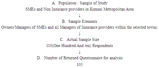
3.4. Sampling Technique

In a sample, each population element was selected individually, (Cooper and Schindler, 2003). The researcher divided the population into clusters for random sampling. The aim of probability sampling was to obtain a subset of a population that was representative of the population. The procedure was useful for the researcher who had little or no knowledge about the population that might be dealt with to avoid any bias. Following from above, the technique was via cluster sampling. The significance of this was that it provided suitability for the study due to heterogeneity between subgroups and homogeneity within subgroups. The SMEs were sampled into clusters according to the number of employees as this was consistent with the classification of SMEs per the GSS definition. The different clusters had SMEs that had the same number of employees as one cluster, one cluster contained small businesses and the other had medium sized businesses as illustrated:

Table 2. Classifications of SMEs Using Headcount

3.5. Methods of Data Analysis

Analysis of data is a process of editing, cleaning, transforming, and modeling data with the goal of highlighting useful information, suggestion, conclusions, and supporting decision making. (Adèr, 2008). Data from the field were edited and coded appropriately to make meaning out of them. Editing was done to correct errors, check for non-responses, accuracy and corrects answers. Coding was done to facilitate data entering and a comprehensive analysis. Descriptive statistics was the medium used for analysis. The software was the Statistical Package for Social Science version sixteen (SPSS 16). Descriptive statistics analysis factors like frequency tables, percentages, pie charts, bar graphs pictures were generated and statistical model logistical regression was used and their interpretations thoroughly explained.

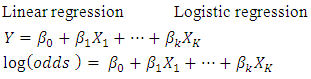
3.6. Logistic Regression

Both linear and logistic regressions analyze the relationship between multiple independent variables and a single dependent variable. However, linear regressions analyze linear relationships, which require a numerical dependent variable (such as age) that follows a normal distribution. In contrast, logistic regressions require binary dependent (categorical) variables, thus variables with two categories. Like dummy variables, these are coded 0/1 and indicate if a condition is or is not present, or if an event did or did not occur. Because there are only two values of the dependent variable (which we will call occurrence or non-occurrence), predicting the probability of occurrence is theoretically interesting. Logistic regressions find the relationship between the independent variables and a function of the probability of occurrence. This is the logit function (hence the name logistic regression), also called the log-odds function. It is the natural logarithm of the odds of occurrence. As it turns out, using the log-odds instead of Y on the left hand side of the equation, the right hand side is identical:

SPSS will be able to calculate the coefficients, which are interpreted as similar to linear regression coefficients.

Advantages of logistic regression

Logistic regression is highly effective at estimating the probability that an event will occur. For this reason, it has been applied to medical research, where it is used to estimate the likelihood of individuals recovering from surgery. Logistic regression differs from other analytic techniques in a number of ways. As the above examples indicate, logistic regression creates for the likelihood that an event occurs, given a set of conditions. This is something that a logistic regression can test.

Logistic regression offers the same advantages as linear regression, including the ability to construct multivariate models and include control variation. It can perform analysis on two types of independent variables - numeric and dummy variables - just like linear regression. In addition, logistic regressions offer a new way of interpreting relationships by examining the relationships between a set of conditions and the probability of an event occurring.

Assumptions of Logistic Regression

i. Logistic regression does not assume a linear relationship between the dependent and independent variables.

ii. The dependent variable must be a dichotomy (2 categories).

iii. The independent variables need not be interval, nor normally distributed, nor linearly related, nor of equal variance within each group.

iv. The categories (groups) must be mutually exclusive and exhaustive; a case can only be in one group and every case must be a member of one of the groups.

v. Larger samples are needed than for linear regression because maximum likelihood coefficients are large sample estimates. A minimum of 50 cases per predictor is recommended. Likewise, a highly skewed numeric variable is not well suited to linear regression analysis, because linear regression requires a normal distribution.

Relationships through Probabilities

Logistic regressions predict likelihoods, measured by probabilities, odds, or log-odds. Often people speak of “probabilities” and “odds” as being the same thing, but there is an important distinction. A probability is the ratio of the number of occurrences to the total number of possibilities. It is easy to convert back and forth between probability and odds, as they give the same information.

Probabilities range from 0 to 1, whereas odds range from 0 to infinity. An odds of one indicates equal probability of occurrence and non-occurrence (0.50). An odds greater than 1 indicates that occurrence is more likely than non-occurrence. An odds less than 1 indicates that occurrence is less likely than non-occurrence. Distinguishing probabilities from odds is very important, not only for accuracy in reporting findings, but also for the interpretation of the logistic regression coefficients and graphs that we will be creating. Note here that even when findings are reported as odds, they can be converted to probabilities using the following formula:

Probability

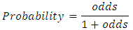or

P: probability of Y occurring

e: natural logarithm base

b₀: interception at y-axis

b₁: line gradient

b_n: regression coefficient of Xn

X₁: predictor variable

X₁ predicts the probability of Y

Log of the Odds and the odds ratio

The Logits (log-odds) are the b coefficients (the slope values) of the regression equation.

The slope can be interpreted as the change in the average value of Y, from one unit of change in X. Logistic regression calculates changes in the log-odds of the dependent, not changes in the dependent value as OLS regression does. For a dichotomous variable the odds of membership of the target group are equal to the probability of membership in the target group divided by the probability of membership in the other group. Odds value can range from 0 to infinity and tell you how much more likely it is that an observation is a member of the target group rather than a member of the other group. Another important concept is the odds ratio (OR), which estimates the change in the odds of membership in the target group for a one unit increase in the predictor. It is calculated by using the regression coefficient of the predictor as the exponent.

Omnibus Tests of Model Coefficients

The overall significance is tested using the Omnibus tests of Model Coefficients, which is derived from the likelihood of observing the actual data under the assumption that the model that has been fitted is accurate. There are two hypotheses to test in relation to the overall fit of the model:

Test of Significance

Hosmer and Lemeshow test

An alternative to model chi square is the Hosmer and Lemeshow test which divides subjects into 10 ordered groups of subjects and then compares the number actually in the each group (observed) to the number predicted by the logistic regression model (predicted). The 10 ordered groups are created based on their estimated probability; those with estimated probability below 0.1 form one group, and so on, up to those with probability 0.9 to 1.0. Each of these categories is further divided into two groups based on the actual observed outcome variable (success, failure). The expected frequencies for each of the cells are obtained from the model. A probability (p) value is computed from the chi-square distribution with 8 degrees of freedom to test the fit of the logistic model.

If the Hosmer and Lemeshow goodness-of-fit test statistic is greater than 0.05, as we want for well-fitting models, we fail to reject the null hypothesis that there is no difference between observed and model-predicted values, implying that the model’s estimates fit the data at an acceptable level. That is, well-fitting models show non-significance on the Hosmer and Lemeshow goodness-of-fit test. This desirable outcome of non-significance indicates that the model prediction does not significantly differ from the observed.

Test for Goodness of fit under Logistic regression model (Hosmer-Lemeshow test)

H₀: Model fits the data well

H₁: Model does not fit the data well

3.7. Limitations

Given limited time and financial constraints of the researcher thorough follow ups were made to ensure extensive recovery of the questionnaire for the research. There were undue delays in getting responses on time due to the schedule of work, especially owners. Again, some of the respondents (illiterates) had their questionnaire read to them with the help of an interpreter before they could respond. Some respondents were apprehensive about Question 10 (appendix 2). It was stressful combing work, social responsibilities, studies and the research. Some of the respondents saw the exercise as a waste of time as they put it and for that matter were not prepared to compromise few minutes of the precious time as it were to answer the questions.

3.8. Brief Profile of Kumasi Metropolis

Kumasi is located in the transitional forest zone, about 270km north of the national capital, Accra. It covers a total land area of 254 square kilometer, stretching between latitude 6.350 – 6.400 and longitude 1.30° – 1.35°, with an elevation which ranges between 250 – 300 metres above sea level. Kumasi is bounded to the north by Kwabre District, to the east by Ejisu Juabeng District, to the west by Atwima Nwabiagya District and to the south by Bosomtwe-Atwima Kwanwoma District. The average minimum temperature is about 21.5°C and a maximum average temperature of about 30.7°C. The metropolis enjoys a double maxima rainfall regime thus 214.3mm in June and 165.2mm in September.

Figure 1. The Sub- Metropolitan Map of the Kumasi Metropolitan Area. (Source: Town and Country Planning Department, 2017)

The administration and management of Kumasi Metropolis is entrusted with the Kumasi Metropolitan Assembly while the custodianship of the land is held with the Traditional Authority. Traditionally, Kumasi Metropolis is the seat of the “Otumfuo”, the king of the Asante Kingdom. It also serves as capital of the Asante Kingdom, which was founded in 1680’s by King Osei Tutu II, as well as the Ashanti Region. The Local Government Act 462, 1993 and Local Government Legislative Instrument LI 1614, 1989 established the Kumasi Metropolitan Assembly (KMA) to manage the city. Furthermore, these legal frameworks have empowered KMA with legislative responsibilities to promulgate rules and by-laws, giving legal effect to its decisions. The Local Government Act 462 (1993) and legislative instrument LI (1614) has also given authority to KMA to become a Planning Authority to formulate policies, programmes and projects as well as to mobilize resources within its jurisdiction to undertake development projects. Kumasi has 10 sub metros (Refer to Figure 1) which are Bantama, Subin, Manhyia, Oforikrom, Tafo-Pankrono, Nhyiaeso, Kwadaso, Suame, Asokwa and Asawase which serve as a link between the community and the Metropolitan Assembly. They bring the process of decision making to the door steps of the grass roots in society. The Sub Metropolitan District Councils are further sub divided into 24 Town Councils and have a total of 419 Unit Committee.

4. Presentation and Analysis of Data

4.1. Introduction

This chapter dealt with the analysis of data from respondents on the research. It was purely from field survey. This section presented information per appendices one (1) and two (2).

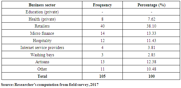
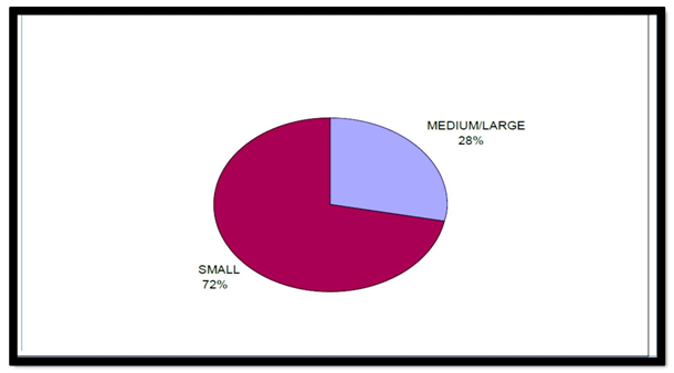
4.2. Types of Business, Ownership and Their Size

Business information was analysed in their fields. First, according to the sector in which they operated and then according to their size.

Table 3. Sectorial involvement of SMEs

Table 3 of the study revealed that the largest type of business in the Kumasi Metropolitan Area is the retail business. This category of business constituted 38.10%, followed by microfinance with 13.3%, and artisans with 12.38%. It further indicated that 11.43% was the Hospitality sector, 7.62% made of private health service providers; 3.81% was made up of internet service providers; washing bay comprised of 2.85%; while other forms of businesses was made up of 10.48%. At the period of data collection, all schools were on Easter break and so no responses were obtained from that sector.

Classification of Business

Businesses were classified according to size and ownership / management.

Source: Researcher’s illustration from field survey, 2017

From figure 2 above, the study indicated that 72% was made of small scale businesses and 28% medium/large scale businesses within the Metropolis that responded to the questionnaire. The information attested to the fact that the small scale sector has the greatest potential of providing jobs to the youth and others in the informal sector of the economy when given the needed support than the formal sector. Following from above, 60% of valid respondents comprised owners of SMEs; 21% were Supervisors; 12% were managers and 7% were only partners. The research indicated that most SMEs were managed by their owners which presupposed that the owners of SMEs were more likely to take business recovery decisions independently.

Type and Locations of Business in Kumasi Metropolis

The locations of businesses were considered under the three constituencies in the Metropolis as indicated on the table 4 below.

Table 4

In respect of table 4 above, the location of respondents comprised: 69% of towns from Kumasi Central Constituency, 19% of towns from Kumai South Constituency and 22% of towns from Kumasi North Constituency. Kumasi Central Constituency had more businesses than the other two. The use of the constituencies was to afford the researcher the opportunity to analyse if possible the types of businesses by location and how if possible that affected their business risk disposition and likelihood of patronizing insurance policy.

Registration of Businesses

The study sought to obtain information on the number of registered businesses that were legally operating in the Metropolis since data was not readily available from the Registrar General Department.

Table 5. Institution of Registered SMEs

Table 5 above shows that 84% of valid responses of SMEs were duly registered with the Registrar General Department; 2% and 1% registered with MASLOC and NBSSI respectively. 13% of SMEs registered with other institutions and those institutions among others included the District Assembly, Domestic Revenue Authority, and Membership Associations of business units and the Tourist Board. SMEs that registered with bodies other than Registrar General Department, obtained: Financial assistance to support their businesses; business operation permit from the Assembly; tax stamp from IRS, permit from Ghana Tourist board (i.e. Hospitality industry) and recognition from membership associations.

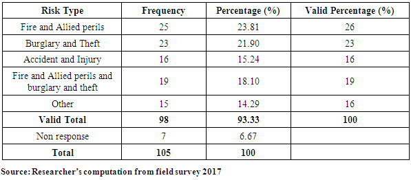
4.3. Analysis of Risk Management

This section analysed the risks that businesses face in Kumasi Metropolis.

Table 6. Risks that Businesses face in Kumasi Metropolis

From table 6 above, 26% of valid respondents were exposed to fire and allied perils; 23% were exposed to burglary and theft; 19% were exposed to burglary, theft, fire and allied perils; while 16% were exposed to accident and injury and 7% represented other that stated particularly speculative risks which were influenced by market conditions. The table reflects that more SMEs were likely to experience fire and allied perils that could affect gravely their business capital and profits. The recent fire outbreaks in the markets such as Asafo market and twice in central market this year 2014 alone, race Course all in Kumasi with some enterprises attested to the high level of business exposures to fire and allied perils that affect property and liability. The stated risk could be categorized into Property Risk, Liability Risk, Income Risk and Personal Risk, as acknowledged by the respondents that they affect negatively their incomes, property, business image, litigation, and socioeconomic livelihood. All 12 but 1 insurance companies’ managers stated the same as above, but added bonds with the exception of speculative risk.

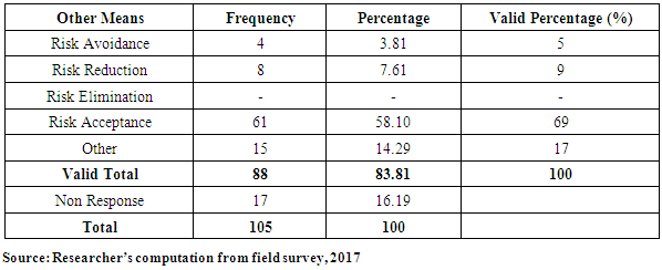
4.4. Management of Business Risks by Entrepreneurs of SMEs

This sought to ascertain the management of risk(s) among SMEs in the Metropolis.

Table 7. The Use of Insurance as a Risk Mitigating Tool

From table 7 above, 58% of the valid respondents agreed and 14% strongly agreed that insurance was a tool for mitigating business risk(s). It was conclusive that more than 58% of the respondents had a positive opinion about insurance as a tool for managing risks. Managers of insurance service providers responded in the affirmative, “yes”; indicating the need to possess insurance policies by business operators. Paradoxically, 84% of valid respondents did not use insurance as a tool for managing business risk(s) (Table 8). Service providers asserted that the level of patronage was low and indicated that of those SMEs that insure, in most cases they under insure. The legislated Insurance Act, 2006 was not duly enforced and so most entrepreneurs resorted to risk acceptance as a management mechanism (table 8) despite its uneconomical implications. Of the 84% who do not use insurance to manage risk(s), 69% of valid respondents adopted risk(s) acceptance; 9% adopted risk reduction and 5% avoided risk(s).

Table 8. Other Business risk(s) management tools

Following from above, a relationship between educational level of entrepreneurs and insurance usage that connoted the irony of the management of business risk(s) regarding insurance was illustrated as below. From table 9, the study revealed that majority of owners obtained Secondary school and Tertiary education respectively; with marginal figures representing College, Primary and Other. Again, the table presented a discouraging relationship between the educational level of owners and its influence on the choice of using insurance. Apart from the college level entrepreneurs that had 71% positive response and except others, the rest had less than 29% “yes” response. Rather, secondary and tertiary levels respectively had 79.6% and 78.6% negative response to using insurance to manage business risk(s). Overall, 71% against 27% do not use insurance. Majority of owners/managers of SMEs who had obtained secondary and Tertiary educational levels, respectively were thought to be better informed to know the hazards that negatively affected business profits and to adopt pragmatic insurable measures to combat such hazards that manifested into losses. The reason for that outcome could be linked to the following: the non-experience of a risk, low level of vulnerability, the negative perception about insurance and the risk acceptance attitude.

Table 9. Relationship between Educational Levels of Entrepreneurs and Insurance Usage

However, the above relationship could only be influenced positively if owners of SMEs required loans from banks that demanded insurance on their collateral as a pre-requisite to the approval of a credit facility. Unfortunately, most of those compelled under the circumstance did not renew their policy covers when they expired.

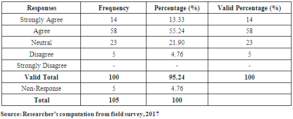
4.5. Benefits of Insurance

The researcher sought to obtain from respondents the benefits that they have had for taking the appropriate insurance covers.

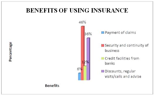Source: Researcher’s illustration from field survey 2017

Figure 3 revealed the following statistics: thirty three (33) respondents to the above theme representing 19% indicated that they benefited variously from insurance policies and companies. Of the respondents, 6% benefited from claim settlement by insurers, 46% benefited from security and business continuity in the events of mishaps to their businesses, 12% were supported obtain credit facilities from financial institutions and 36% gained discounts on premiums, souvenirs, regular visits, call from some insurers and prudent business advice. In addition, they benefited from professional advice on due diligence and how to manage stock updates for safety of assets and investments.

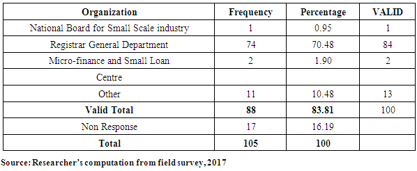
4.6. Information on Insurance

The level of patronage of insurance might depend on the level of information available to owners/managers of SMEs on the need to select the appropriate insurance policies.

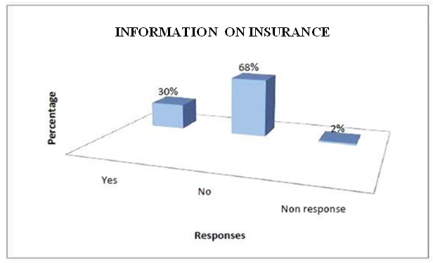Source: Researcher’s illustration from field survey 2017

From figure 4 above, 68% of respondents answered in the negative, while only 30% responded positively to having enough information to choose appropriate insurance policy or policies. This was in conformity with table 9. The low level of insurance patronage might be due to information asymmetry and other associated factors.

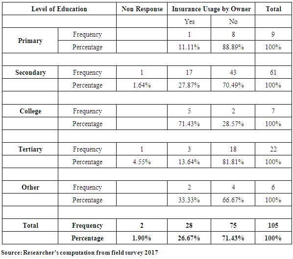
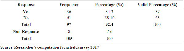
4.6.1. Awareness of Compulsory Insurance

The level of awareness of the insurance Act was to drum home the legal need to have property and liability insurance to enhance the level of response and patronage Table 10: Awareness level of compulsory fire and liability insurance.

Table 10

Table 10 above, illustrated that less than 37% valid respondents were aware of the mandated fire and liability insurance enacted in 2006, Act 724, sections 183 and 184. The situation called for the industry players to team up with the appropriate agencies, especially the regulatory body to enhance its education and significance.

4.7. Challenges of Businesses Using Insurance

This sought to ascertain the challenges that SMEs were likely to face with insurance companies.

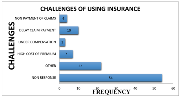Source: Researcher’s computation from field survey 2017

From figure 5 above, of the total respondents of 46, representing 44% of sample size of SMEs: 4 indicated non-payment of claims: 10 indicated delay claim payment; 3 indicated under compensation of claim; 7 acknowledged high cost of premium; and, 22 other stated delayed renewal notice and policy delivery. However, service providers in the industry thought otherwise and stated that appropriate compensations were paid to claimants who had appropriate insurance covers. Again, considering the risk factors that surround the business environment premiums were such charged appropriately.

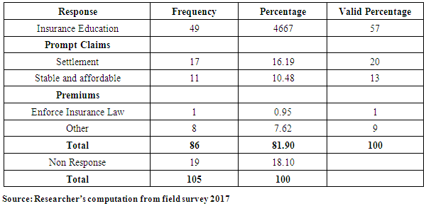
4.8. Suggested Solutions to Challenges to Using Insurance

The respondents were asked to suggest solutions to problems that they encountered with their insurers in terms of service delivery.

Table 11. Solutions to Challenges

From table 11 above, 57% of the valid respondents representing the majority applauded insurance education to be enhanced. 20% advocated prompt payment of claims. 13% indicated that the cost of insurance should be made affordable and reliable. 1% called for the enforcement of the insurance law; while 9% representing other appealed to insurance companies to provide loans to SMEs.

4.9. Detailed Analysis

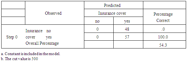
4.9.1. Beginning Block

The beginning block presents the results with only the constant included before any coefficients of the independent variables are entered into the equation. Logistic regression compares this model with a model including all the predictor to determine whether the latter model is more appropriate.

Table 12. Beginning Classification Table

The classification above, suggests that if we knew nothing about our variables and guessed that the individual (SME) will opt for an insurance cover we would be correct 54.3% of the time.

Table 13. Variables in the Equation

For the constant term only model, the constant term with a value of 0.172 with a corresponding p- value of 0.380 implies that it not is significant in the logistic model in determining whether the individual will go for an insurance cover or not.

Block 1 Method

This presents the results when the predictors are included. By adding the variables we can now predict with 81.6% accuracy (Table 14). The model appears good, but we need to evaluate model fit and significance as well. With the statistical tests for model fit and whether each of the independent variables included make a significant contribution to the model.

Table 14. Classification

The overall accuracy of the classification from the table 14 of 68.6% is greater than the classification accuracy in the beginning (Table 15). From literature the final classification accuracy should always be 25% more than the classification accuracy at the beginning block 0 for good model.

Table 15. Omnibus Tests of Model Coefficients

Model chi-square.

The overall significance is tested using the Omnibus tests of Model Coefficients, which are derived from the likelihood of observing the actual data under the assumption that the model that has been fitted is accurate. There are two hypotheses to test in relation to the overall fit of the model:

Versus

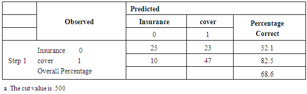
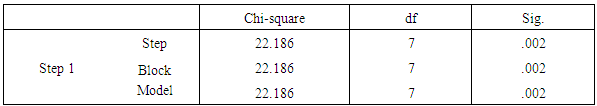
From the chi-squared value of 22.187, degrees of freedom 7 and significance value of 0.002 leads to the rejection of the null hypothesis and concluding that the model coefficients are significantly different from zero.

Hosmer and Lemeshow

This is a reliable goodness of fit test of the model in Spss output. The model is a good- fit of the data when the significance value is greater than 0.05.

Hypothesis testing

The model fits the data

The model does not fit the data

Table 16. Hosmer and Lemeshow Test

From the table above, the Hosmer and Lemeshow p-value of 0.630 is greater than the alpha value, Therefore the null hypothesis is not rejected and we conclude that, the observed numbers of households are not significantly different from those predicted by the model and hence the overall model is a good fit of the data.

Table 17. Variables in the Equation

The Variables in the Equation table above has several important elements. The Wald statistic and associated probabilities provide an index of the significance of each predictor in the equation.

Hence, we reject the null hypothesis and conclude that the variables make significant contribution to the model.

The exp (B) column in Table presents the extent to which raising the corresponding measure by one unit influences the odds ratio.

The “B” values are the logistic coefficients that can be used to create a predictive equation (similar to the b values in linear regression). In this example:

Where,

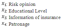
5. Findings, Conclusions and Recommendations

5.1. Introduction

This chapter presented the findings and conclusions arrived at in the research. It also dealt with suggestions/recommendations based on the study.

5.2. Summary of Findings

The following were the findings obtained from the survey. The study showed that businesses were exposed to the following business risks: Fire and allied perils, Burglary and theft, Accident and injury that affected their business operations. These were variously classified by the findings as property and liability risk, income risk and personal risks respectively. Given the paradox, the study showed that, 84% of valid respondents expressed their opinions in favour of insurance as a tool for mitigating business risk(s); the level of insurance patronage was relatively low in the Metropolis. The majority adopted risk acceptance as a form of managing business risk. The research revealed the following as benefits derived from using insurance as a risk mitigating tool: payment of claims for insured risk(s) for business recovery, provision of security and peace of mind, provision of renewal premium discounts, regular visits to clients by some insurers, provision of aid to facilitating credit facilities from banks at moderate interest rates and professional advice on due diligence.

The study found the following as some challenges that insured SMEs faced using insurance: delay in claim settlement due to bureaucratic process, incomplete compensation to SME claimants, high cost of risk transfer (i.e. high premiums), late delivery of renewal notices, technical and complex terms of reference with hidden contractual clauses and short circuiting of information and education from agents. Recommended solutions from the study were identified as follows: enhancement of insurance education, prompt payment of claims, affordable or stable premiums charges for appropriate risk(s).

Furthermore, the research showed that SMEs did not have appropriate insurance covers to manage their risk(s). Of those who insured, many under insured to pay less premiums. Again, the work showed that the awareness level of the compulsory fire and liability insurance section in the insurance Act, 2006 was marginal. Many SMEs were not familiar and only got informed during the survey. This act was not enforced; that could have also accounted for the inadequacies of their risk recovery response. The findings revealed that most SMEs demanded insurance for stock in trade and mortgage only when required by financial institutions as a pre-requisite to loan approval and disbursement. However, a few were compelled by a partner company to buy insurance.

5.3. Conclusions

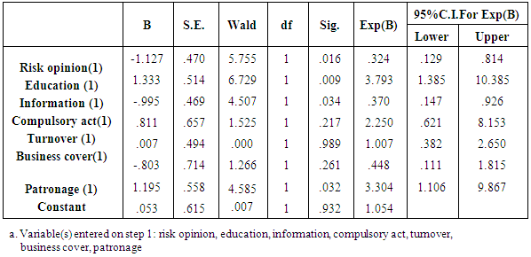
In conclusion, the study generally revealed that: business risk(s) exposures were identified and classified under three main themes;

Ÿ The level of insurance patronage was relatively low; however,

Ÿ Insured businesses derived various benefits under the insurance covers.

Ÿ The insured also encountered some challenges, but made some suggestions to help overcome those problems.

Ÿ For an SME to opt in for an insurance cover, it will depend on the

Ÿ Attitude to risk (Risk Opinion)

Ÿ Educational Level

Ÿ Information on insurance

Ÿ Level of patronage

Ÿ The model can be used to predict likelihood of SME‟s going in for insurance covers

5.4. Suggestions/Recommendations

1. The best ingredient is to engage SMEs and Insurance companies as well as insurance intermediaries to encourage motivating business rapports where SMEs can easily have access to risk management information and insurance policy covers discussed to avert any unforeseen business operational calamities such as what occurred at the Tema Oil Refinery, Kumasi Central Market, Race Course all just this year 2014.

2. Further studies could be made to improve the model.

3. Furthermore, an improved and monitored decentralized claim settlement system should be incorporated to reduce the high level of bureaucracy and delays involved in claims processing by insurance companies.

4. An enforcement of the fire and liability insurance will have positive externalities on businesses and the economy at large. There will be increased comprehensive protection for SMEs and large businesses; premium income of the insurance industry will increase; tax revenue to government will increase; there will be an increase in corporate social responsibility offered to communities; employment level will be enhanced; and it will help increase and sustain the capitalization level of the insurance industry.

Entrepreneurs of SMEs require to be educated on the need to have insurance and appropriate insurance to recover business losses associated with their operations. The need for periodic workshops to be organized by industry players for SMEs is vital to explaining the cost of insurance and measures by SMEs to reduce insurance cost. There is the need for SMEs to change their risk acceptance attitude to embrace insurance in other to avert using funds not allocated for business losses resulting from hazardous events. Failure to embrace insurance as a tool agreed by almost every SME may result in the business not being able to recover from crises. Such affects business reputation, survival and continuity or even the loss of customers thus affecting profit. Given the features of SMEs, their risks vary and the ability to afford the cost of insurance might be a challenge. Full needs assessment is therefore required to design customer made/customized policies that best suit the needs of SMEs independently since there are different potentials in different sectors of their operations. With regards to premium payment, a payment plan could be designed for special needs of SMEs over a period. The compulsory fire and liability insurance Act requires government and the umbrella body of insurance companies to enforce the laws as done for the motor traffic Act of 1985, (Act 42); and insurance stickers (certificate) designed for it. General insurance companies may form strategic alliance with financial institutions to educate and provide SMEs insurance covers and payment channelled through the financial institutions that are least likely to default.