1. Introduction

Ann is a simplified mathematical model of the human brain. It can be implemented by both electric elements and computer software. It is a parallel distributed processor with large numbers of connections; it is an information processing system that has certain performance characters in common with biological neural networks. Ann has been developed as generalizations of mathematical models of human cognition or neural biology, based on the assumptions that:

1- Information processing occurs at many simple elements called neurons that are fundamental to the operation of Ann's.

2- Signals are passed between neurons over connection links.

3- Each connection link has an associated weight which, in a typical neural net, multiplies the signal transmitted.

4- Each neuron applies an action function (usually nonlinear) to its net input (sum of weighted input signals) to determine its output signal [15].

The units in a network are organized into a given topology by a set of connections, or weights.

Ann is characterized by [28]:

1- Architecture: its pattern of connections between the neurons.

2- Training Algorithm: its method of determining the weights on the connections.

3- Activation function.

Ann are often classified as single layer or multilayer. In determining the number of layers, the input units are not counted as a layer, because they perform no computation. Equivalently, the number of layers in the net can be defined to be the number of layers of weighted interconnects links between the slabs of neurons [44].

1.1. Multilayer Feed Forward Architecture [21]

In a layered neural network the neurons are organized in the form of layers. We have at least two layers: an input and an output layer. The layers between the input and the output layer (if any) are called hidden layers, whose computation nodes are correspondingly called hidden neurons or hidden units. Extra hidden neurons raise the network’s ability to extract higher-order statistics from (input) data.

The Ann is said to be fully connected in the sense that every node in each layer of the network is connected to every other node in the adjacent forward layer; otherwise the network is called partially connected. Each layer consists of a certain number of neurons; each neuron is connected to other neurons of the previous layer through adaptable synaptic weights w and biases b.

1.2. Literature Review

Pan and Duraisamy in 2018 [31] studied the use of feedforward neural networks (FNN) to develop models of non-linear dynamical systems from data. Emphasis is placed on predictions at long times, with limited data availability. Inspired by global stability analysis, and the observation of strong correlation between the local error and the maximal singular value of the Jacobian of the ANN, they introduced Jacobian regularization in the loss function. This regularization suppresses the sensitivity of the prediction to the local error and is shown to improve accuracy and robustness. Comparison between the proposed approach and sparse polynomial regression is presented in numerical examples ranging from simple ODE systems to nonlinear PDE systems including vortex shedding behind a cylinder, and instability-driven buoyant mixing ow. Furthermore, limitations of feedforward neural networks are highlighted, especially when the training data does not include a low dimensional attractor. The need to model dynamical behavior from data is pervasive across science and engineering. Applications are found in diverse fields such as in control systems [41], time series modeling [37], and describing the evolution of coherent structures [12]. While data-driven modeling of dynamical systems can be broadly classified as a special case of system identification [23], it is important to note certain distinguishing qualities: the learning process may be performed off-line, physical systems may involve very high dimensions, and the goal may involve the prediction of long-time behavior from limited training data. Artificial neural networks (ANN) have attracted considerable attention in recent years in domains such as image recognition in computer vision [18, 35] and in control applications [12]. The success of ANNs arises from their ability to effectively learn low-dimensional representations from complex data and in building relationships between features and outputs. Neural networks with a single hidden layer and nonlinear activation function are guaranteed to be able to predict any Borel measurable function to any degree of accuracy on a compact domain [16]. The idea of leveraging neural networks to model dynamical systems has been explored since the 1990s. ANNs are prevalent in the system identification and time series modeling community [20, 26, 27, 33], where the mapping between inputs and outputs is of prime interest. Billings et al. [5] explored connections between neural networks and the nonlinear autoregressive moving average model (NARMAX) with exogenous inputs. It was shown that neural networks with one hidden layer and sigmoid activation function represent an infinite series consisting of polynomials of the input and state units. Elanayar and Shin [13] proposed the approximation of nonlinear stochastic dynamical systems using radial basis feedforward neural networks. Early work using neural networks to forecast multivariate time series of commodity prices [9] demonstrated its ability to model stochastic systems without knowledge of the underlying governing equations. Tsung and Cottrell [42] proposed learning the dynamics in phase space using a feedforward neural network with time-delayed coordinates. Paez and Urbina [29, 30, 43] modeled a nonlinear hardening oscillator using a neural network-based model combined with dimension reduction using canonical variate analysis (CVA). Smaoui [38, 39, 40] pioneered the use of neural networks to predict fluid dynamic systems such as the unstable manifold model for bursting behavior in the 2-D Navier-Stokes and the Kuramoto-Sivashinsky equations. The dimensionality of the original PDE system is reduced by considering a small number of proper orthogonal decomposition (POD) coefficients [4]. Interestingly, similar ideas of using principal component analysis for dimension reduction can be traced back to work in cognitive science by Elman [14]. Elman also showed that knowledge of the intrinsic dimensions of the system can be very helpful in determining the structure of the neural network. However, in the majority of the results [38, 39, 40], the neural network model is only evaluated a few time steps from the training set, which might not be a stringent performance test if longer time predictions are of interest. ANNs have also been applied to chaotic nonlinear systems that are challenging from a data-driven modeling perspective, especially if long time predictions are desired. Instead of minimizing the pointwise prediction error, Bakker et al. [3] satisfied the Diks’criterion in learning the chaotic attractor. Later, Lin et al. [21] demonstrated that even the simplest feedforward neural network for nonlinear chaotic hydrodynamics can show consistency in the time-averaged characteristics, power spectra, and Lyapunov exponent between the measurements and the model. A major difficulty in modeling dynamical systems is the issue of memory. It is known that even for a Markovian system, the corresponding reduced-dimensional system could be non-Markovian [10, 32]. In general, there are two main ways of introducing memory effects in neural networks. First, a simple workaround for feedforward neural networks (FNN) is to introduce time delayed states in the inputs [11]. However, the drawback is that this could potentially lead to an unnecessarily large number of parameters [19]. To mitigate this, Bakker [3] considered following Broomhead and King [6] in reducing the dimension of the delay vector using weighted principal component analysis (PCA). The second approach uses output or hidden units as additional feedback. As an example, Elman’s network [19] is a recurrent neural network (RNN) that incorporates memory in a dynamic fashion. Miyoshi et al. [24] demonstrated that recurrent RBF networks have the ability to reconstruct simple chaotic dynamics. Sato and Nagaya [36] showed that evolutionary algorithms can be used to train recurrent neural networks to capture the Lorenz system. Bailer-Jones et al. [2] used a standard RNN to predict the time derivative in discrete or continuous form for simple dynamical systems; this can be considered an RNN extension to Tsung’s phase space learning [42]. Wang et al. [45] proposed a framework combining POD for dimension reduction and long-short-term memory (LSTM) recurrent neural networks and applied it to a fluid dynamic system.

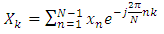
1.3. Fast Fourier Transform

The first to propose the techniques that we now call the fast Fourier transform (FFT) for calculating the coefficients in a trigonometric expansion of an asteroid’s orbit in 1805 [8]. However, Fast Fourier transform is an algorithm that calculates the value of the discrete Fourier transform in faster. the speed this algorithm Is due to the fact that it does not calculate the parts that are equal to zero .the algorithm is discovered by James W. Cooley and John W. Tukey who published the algorithm in 1965 [11]

As know today

(1)

The coefficients can be determined as follows:

(2)

(3)

(4)

The discrete Fourier transform (DFT) is one of the most powerful tools in Digital signal processing. The DFT enables us to conveniently analyze and Design systems in frequency domain [1] and the formal as:

(5)

This paper contains six sections, the first one related with general concepts and some literature review. In the second section, we introduce some properties of Tinkerbill map. The suggested network in details is discussed in section three, while description of the training process for Tinkerbell map is presented in section four. Section five contains the results discussion. Finally, the summary of the research is in section six.

2. Tinkerbell Map [17]

The Tinkerbell two dimensional map is expressed through the following equation:

(6)

Where subscript n represents iteration steps corresponding to the discrete time evolution of the system, and a, b, c, d are parameters. The origin of the name Tinkerbell is unknown; however, the graphical picture of the system shows a similarity to the movement of the Tinkerbell over the Cinderella Castle, as shown at the beginning of the familiar Disney cartoons. The study of map is mathematically fundamental with many practical interests.

The Tinkerbell map for some special cases has been studied; for example, Nusse and Yorke [1997] reported the finding of 64 period-10 unstable periodic orbits and one strange chaotic with a fractal basin boundary at a = 0.9, b = − 0.6013, c = 2, d = 0.5 using a quasi-Newton method on map. Davidchack et al. [2001] implemented the Schmelcher–Diakonos method on map and observed a drastic increase in the number of seeds as the period is increased. 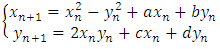In addition, Aulbach and Colonius [1996] provided a figure of pseudo-orbit of length 1 00 000 at a = 0.9, b = − 0.6013, c = 2, d = 0.5 of the map by using the Finite-time Shadowing Theorem [Aulbach & Colonius, 1996].

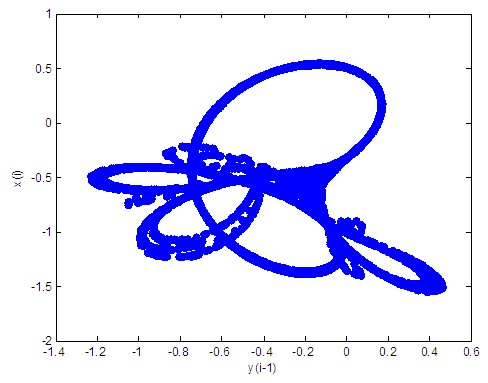Figure 1. Tinkerbell attractor for a = 0.9 and b = -0.6103, c=2, d=0.5

2.1. Tinkerbell Map Solution

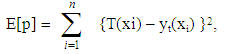
In this section we will explain how this approach can be used to find the approximate solution of the Tinkerbell map that is stated in equation (6).

T(x) is the solution to be computed. Let y_t(x, p) denotes a trial solution with adjustable parameters p.

In the proposed approach, the trial solution y_t employs a FFNN and the parameters p corresponding to the weights and biases of the neural architecture. We choose a form for the trial function y_t(x,p) such that y_t(x,p) = N(x, p) where N(x, p) is a single-output FFNN with parameters (weights) p and n input units fed with the input vector x.

2.2. Computation of the Gradient

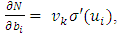
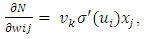
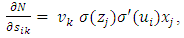
The error corresponding to each input vector x_i is the value E (x_i) which has to force near zero. Computation of this error value involves not only the FFNN output but also the derivatives of the output with respect to any of its inputs. Therefore, for computing the gradient of the error with respect to the network weights, consider a multilayer FFNN with n input units (where n is the dimensions of the domain), two hidden layer with H sigmoid units,q hidden layer and a linear output unit .

For a given input vector x ( x₁, x₂, …, x_n ) the output of the FFNN is:

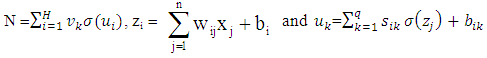w_ij denotes the weight connecting the input unit j to the hidden unit i

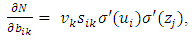
denotes the weight connecting the hidden unit i to the hidden unit k

v_k denotes the weight connecting the hidden unit k to the out put unit,

b_i denotes the bias of hidden unit i,

b_ik denotes the bias of hidden unit i to the hidden unit k, and

σ is the transfer function

The gradient of suggest FFNN, with respect to the coefficients of the FFNN can be computed as:

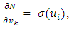(7)

(8)

(9)

(10)

(11)

The derivative of the error performance with respect to the FFNN coefficients can be defined and then it is easy to find minimization solution.

3. Suggested Network

It is well known that a multilayer FFNN consist one hidden layer can approximate any function to any accuracy [25], but dynamical maps they have more completed behavior than other functions, thus, we suggest FFNN contains two hidden layer, one input and one output to estimate a solution for dynamic maps.

The suggested network divided the inputs in to two parts 60% for training and 40% for testing. The error quantity to be minimized is given by:

(12)

Where x_i ∈ [0, 1]. It is easy to evaluate the gradient of the performance with respect to the coefficient. Using (7) – (11). The training progress algorithm of FFNN with supervises training and BFGS algorithm is given as follows. Assume that there are one node in the First layer (input layer), the second layer (hidden layer) consist with ten nodes, the third layer (hidden layer) consist with five nodes and the fourth layer (output layer) consist with one node.

Following the steps of the technique as an algorithm,

Step 0: input and target.

Insert the input (x: x₁, x₂, x₃,…., x_n) and the target.

Step 1: allocating inputs.

Each input goes to each neuron with a hidden layer.

Step 2: initialization weights.

We initial weights and bias from the uniform distribution respectively for all connection in the neural network.

Step 3: select the following.

- parameter epoch

- parameter goal

- performance function (MSE)

Step 4: calculations in each node in the first hidden layer.

In each node in hidden layer, compute the sum of the product of weights and inputs and adding the result to the bias.

Step 5: compute the output of each node for the first hidden layer.

Take the active function for sum value in step4, then its output is sent to the second hidden layer as input.

Step 6: calculations in each node in the second layer.

In each node in second hidden layer, compute the sum of the product of weights and inputs and add the result to the bias.

Step 7: compute the output of each node for the second hidden layer.

Take the active function for sum value in step6, then its output is sent to the output layer as input.

Step 8: calculations in output layer.

There is only one neuron (node) in the output layer. The node sum is the product of weights by inputs.

Step 9: compute the output of node in output layer

The value of active function for node output is also considered as the output of overall network.

Step 10: compute the mean square error (MSE).

The mean square error is computed as follows

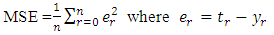the MSE is a measure of performance.

Step 11: The checking.

When such that is small value close to zero, then stop the training and the bias and weights are sent. Otherwise training process goes to the next step.

Step 12: when select the training rule, the low for update weights and bias between the hidden layer and the output layer are calculated

Step 13: the update weights and bias in output layer.

At end for each iteration, the weights and bias are updating as follows:

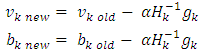When (new) means the current iteration and (old) means the previous iteration,

represents the gradient for weights and bias, is the parameter selected to minimize the performance function along the search direction, represent the invers hessian matrix,v is the weight in the output layer and b is the bias.

Step 14: the update of weights and bias in the first hidden layer.

Each hidden node in the first hidden layer updates the weights and bias as follow:

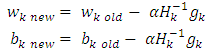Where w is the weight of hidden layer and b is the bias.

Step 15: the update of weights and bias in the second hidden layer as follow.

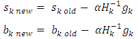Where s is the weight of hidden layer and b is the bias.

Step 16: return to step2 for next iteration.

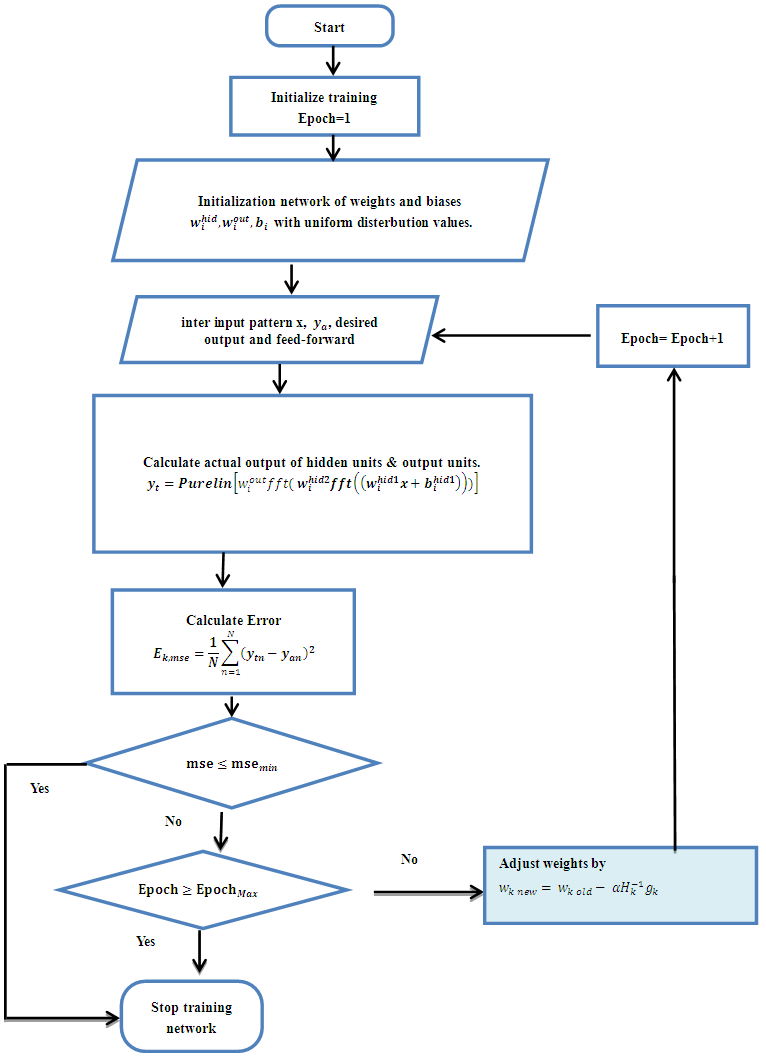Figure 2. Flowchart for training algorithm with BFGS

4. Description of the Training Process for Tinkerbell Map

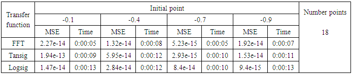
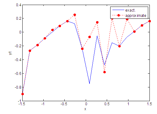
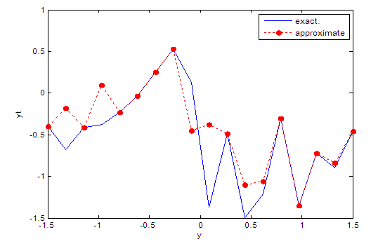
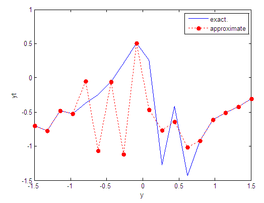
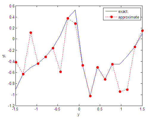
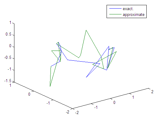
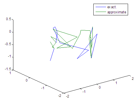
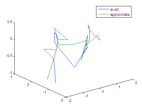
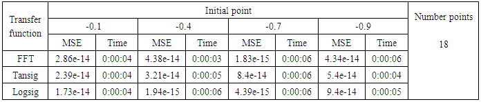
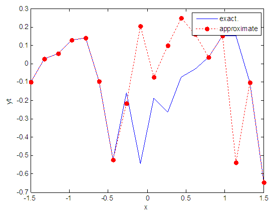
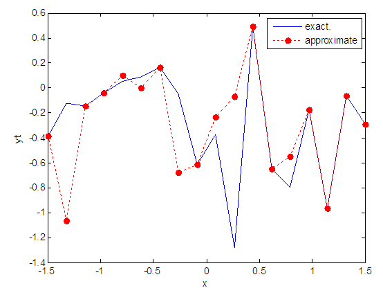
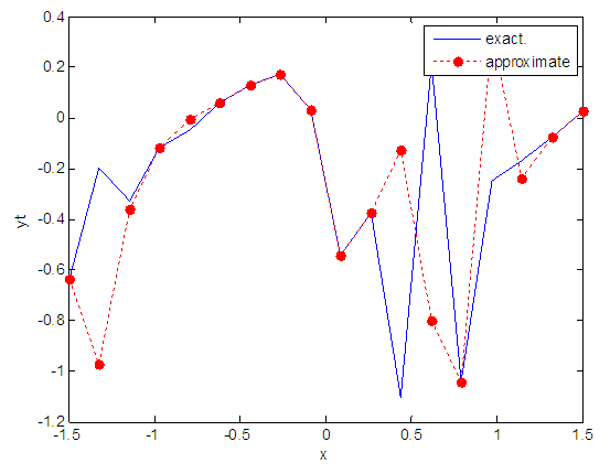
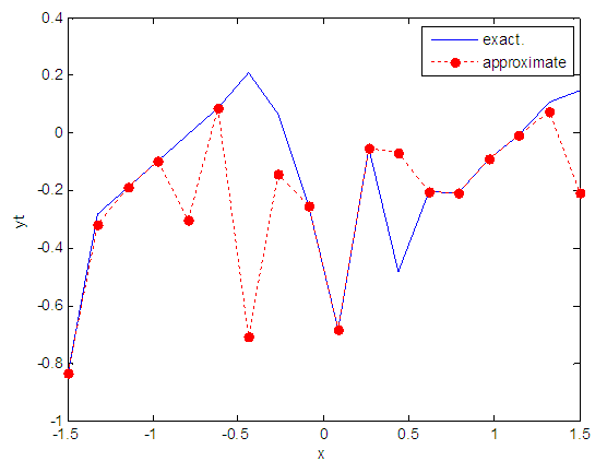
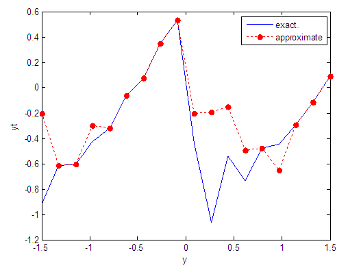
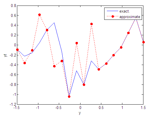
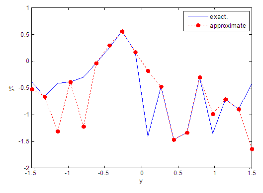
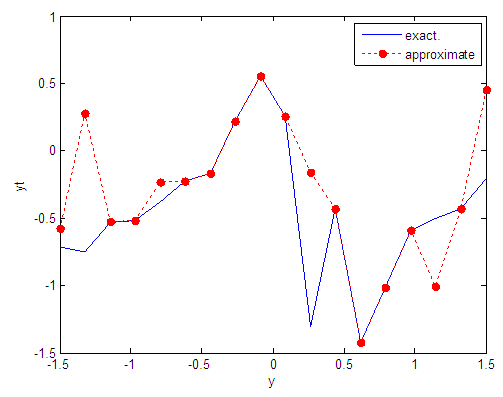
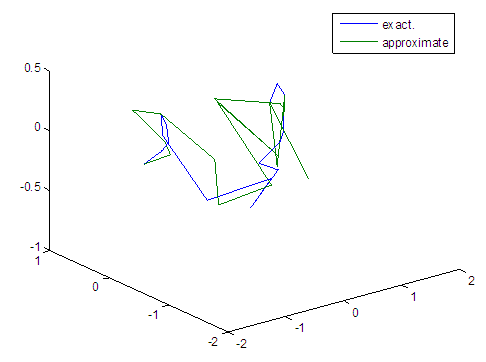
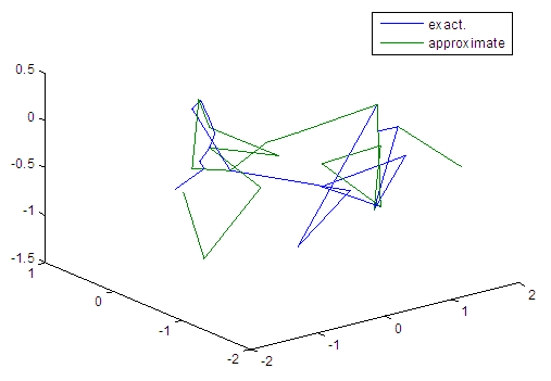
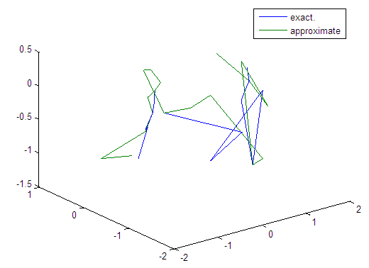
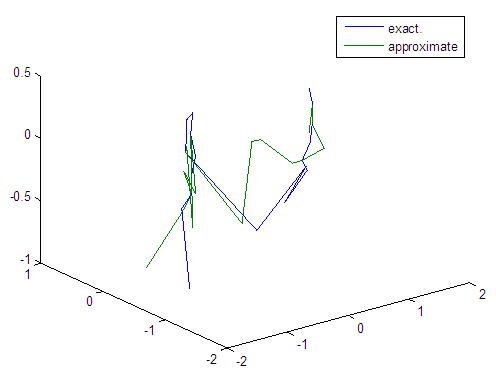
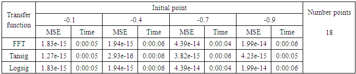
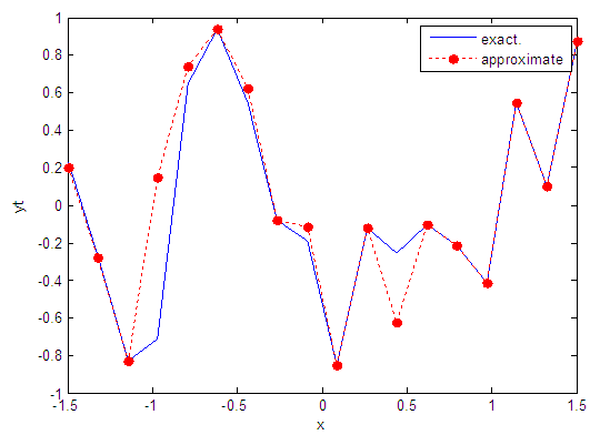
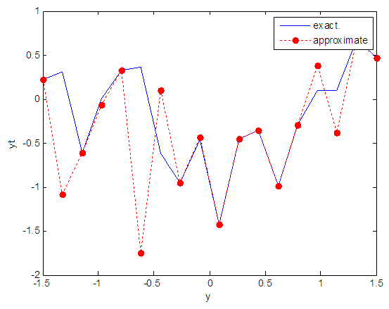
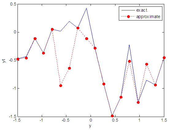
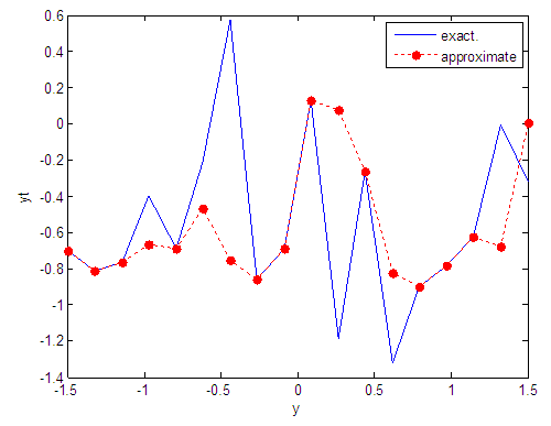
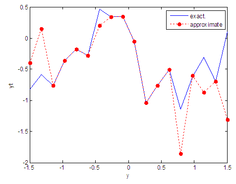
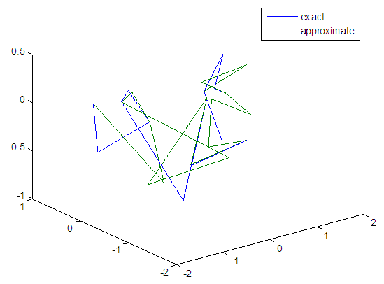
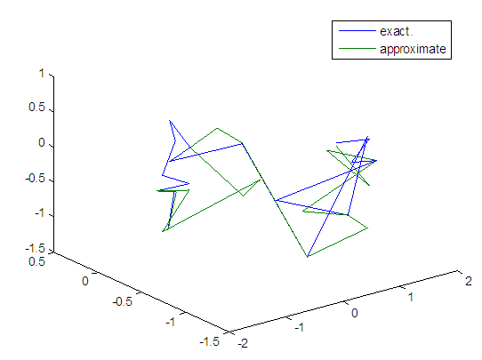
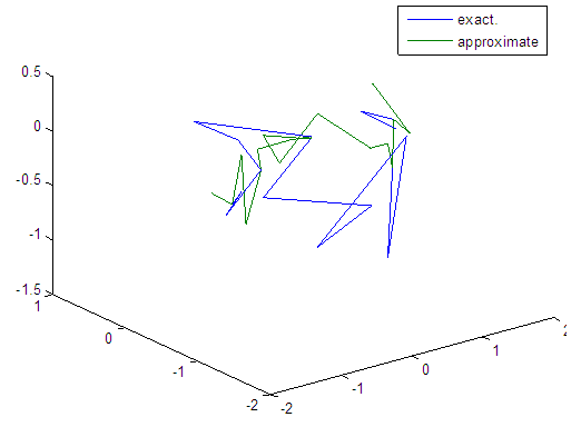
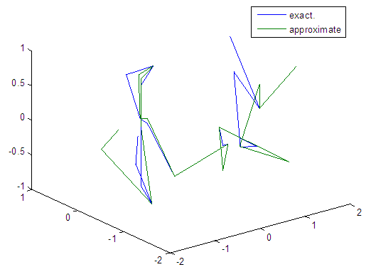
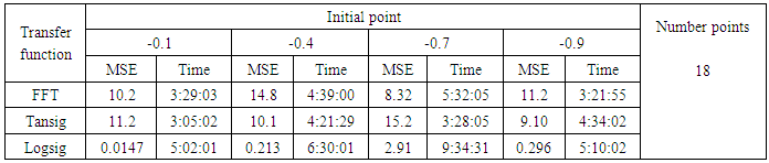
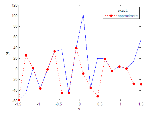
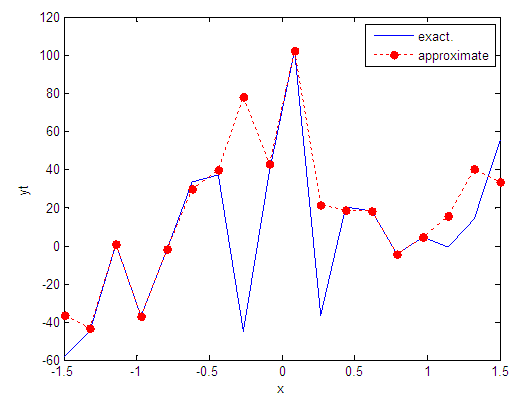
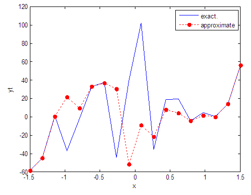
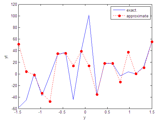
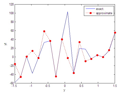
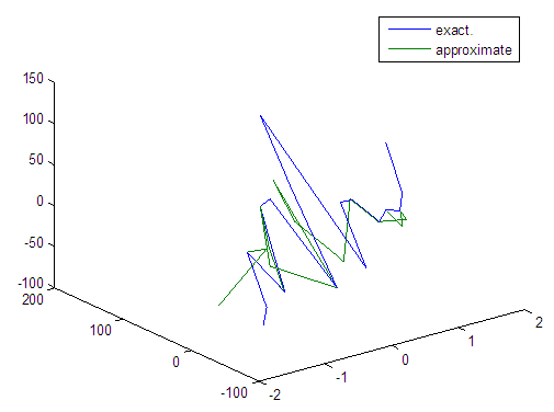
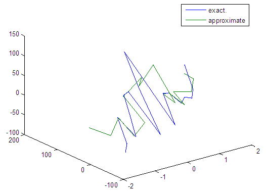
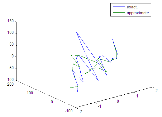
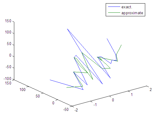
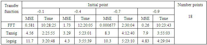
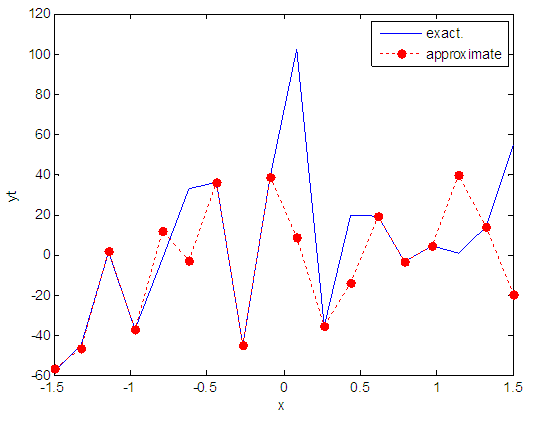
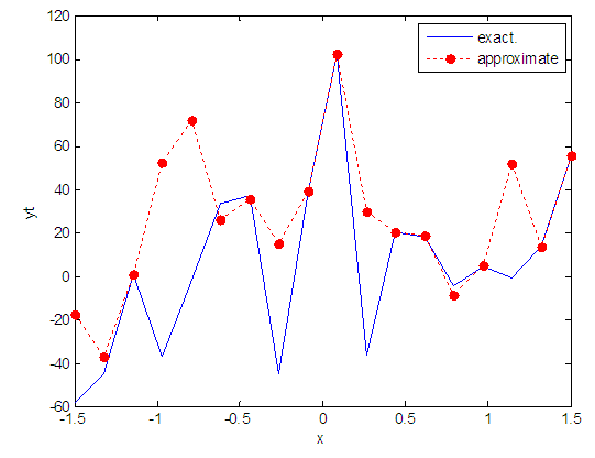
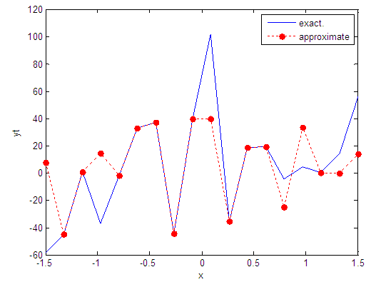
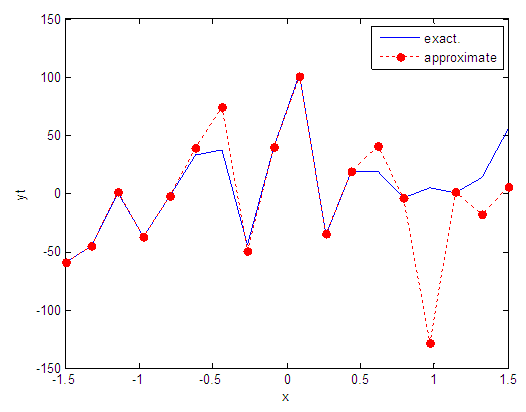
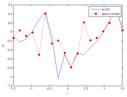
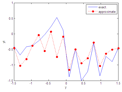
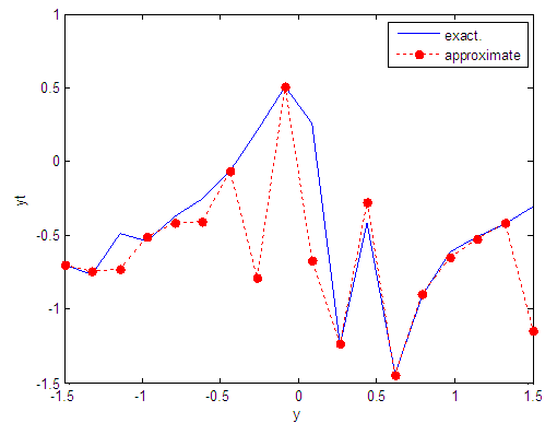
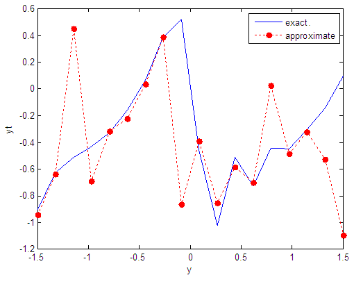
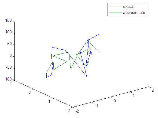
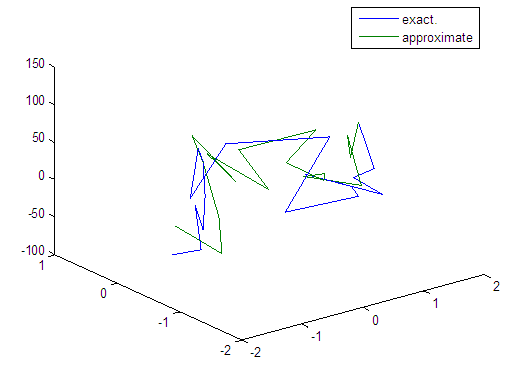
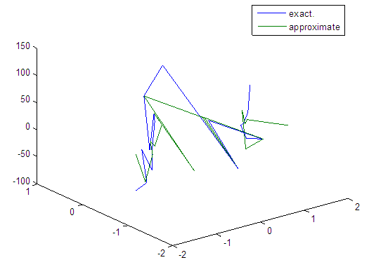
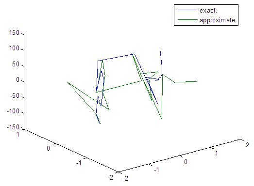
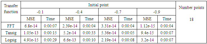
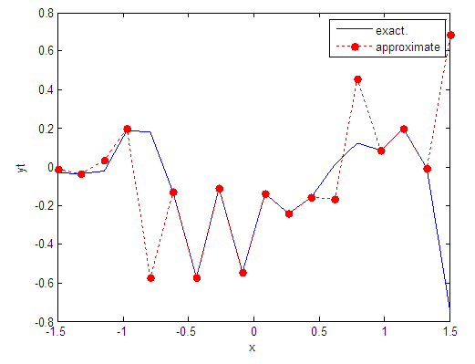
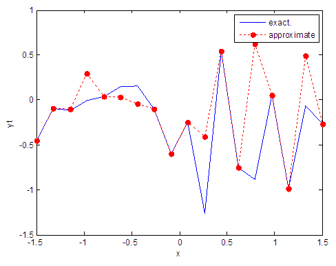
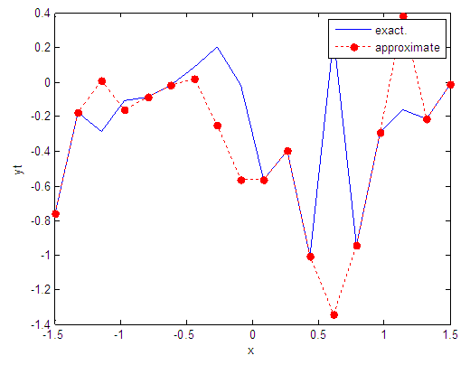
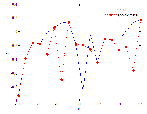
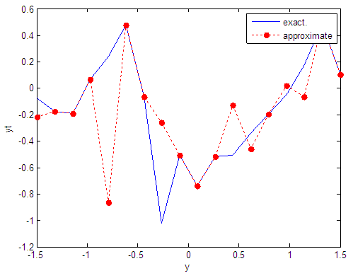
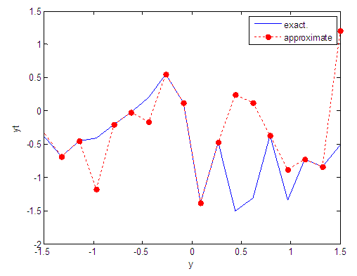
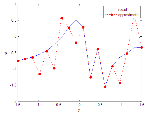
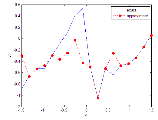
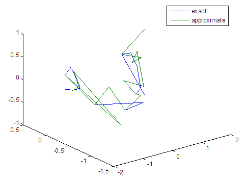
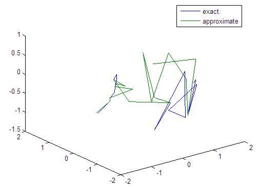
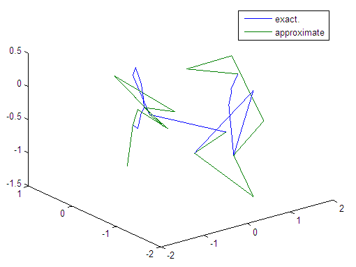
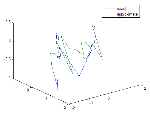
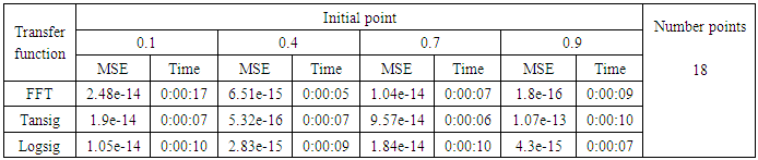
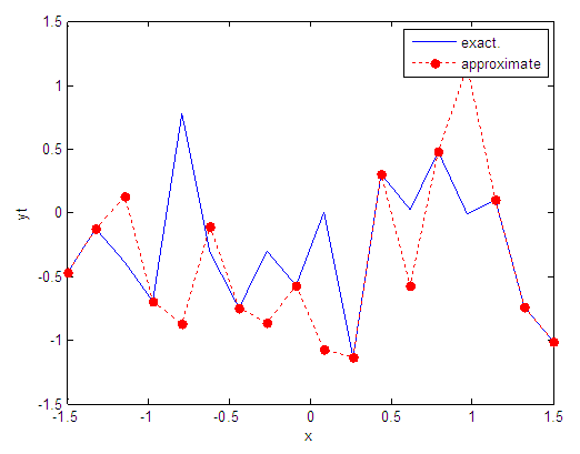
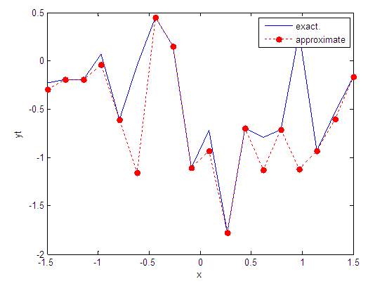
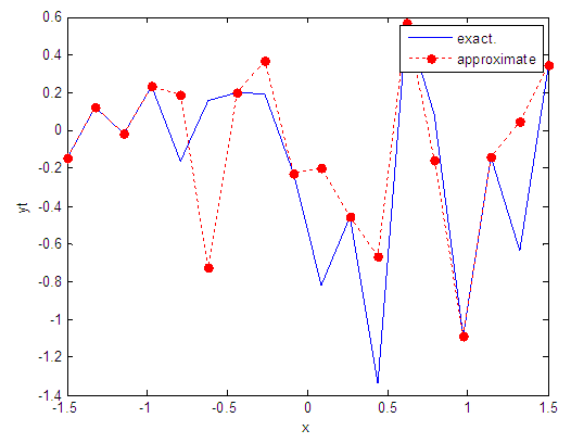
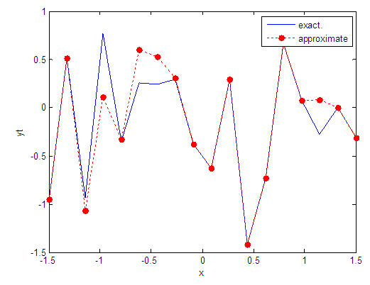
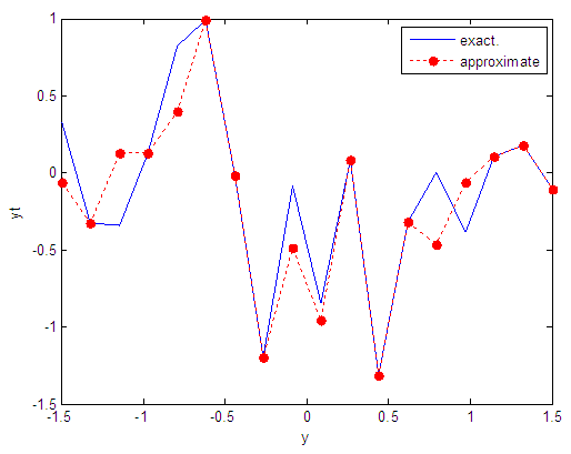
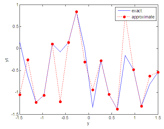
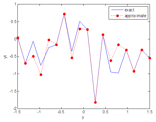
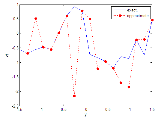
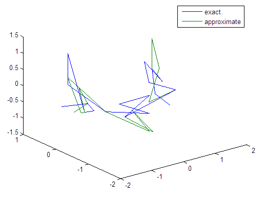
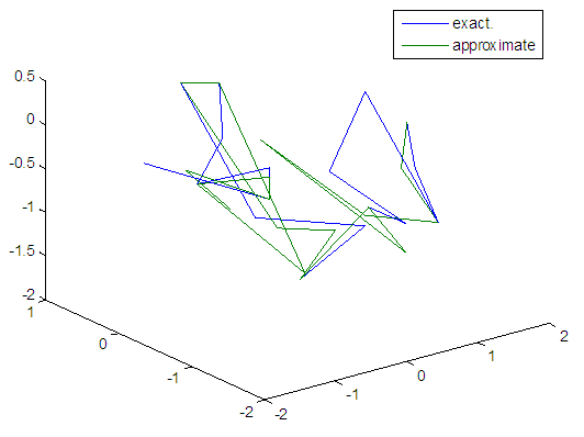
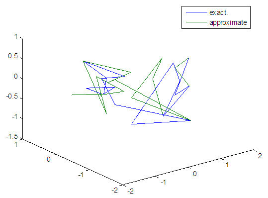
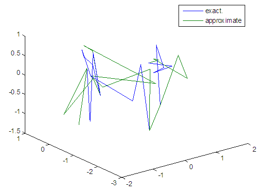
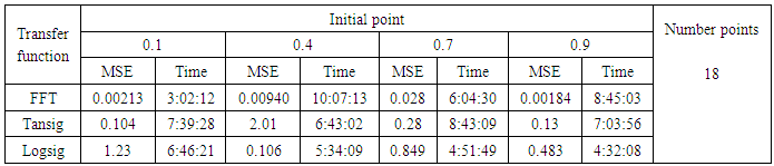
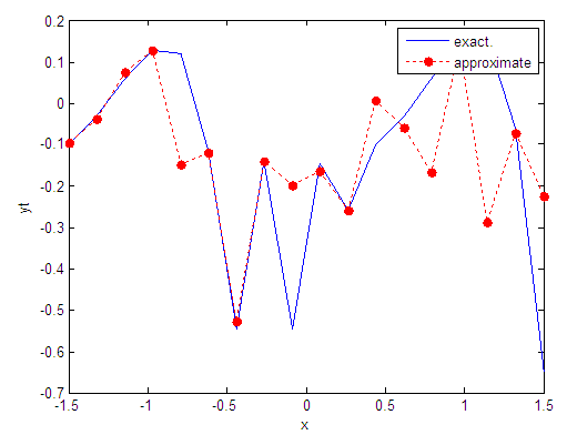
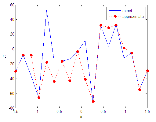
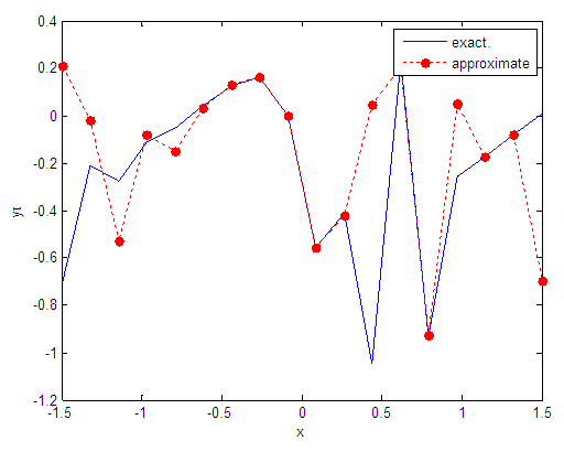
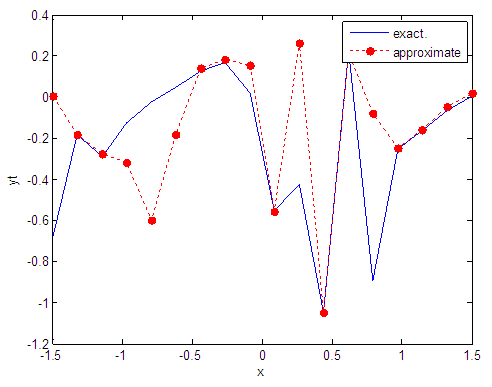
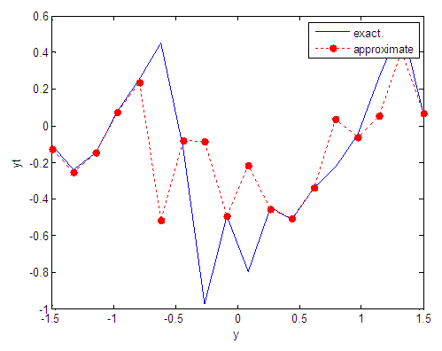
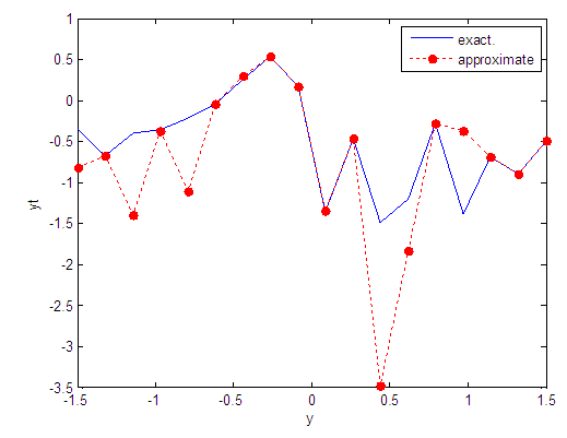
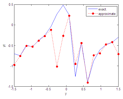
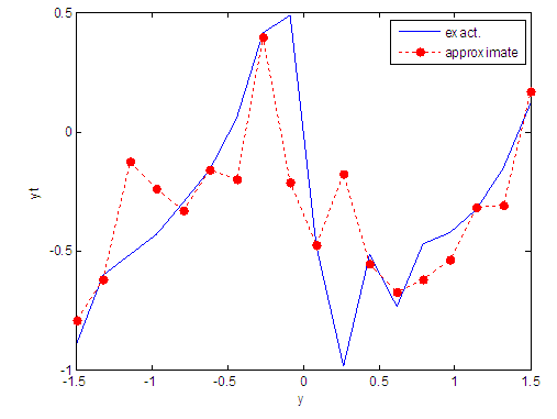
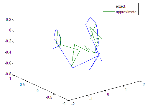
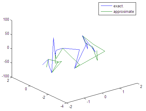
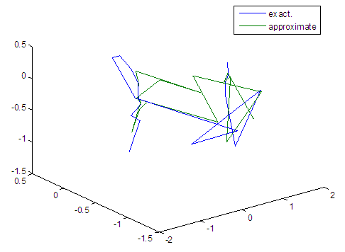
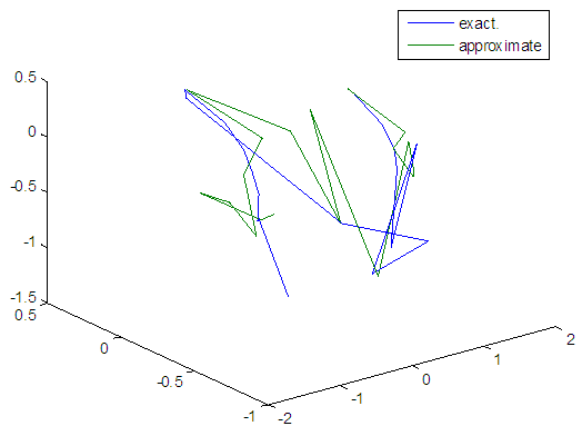
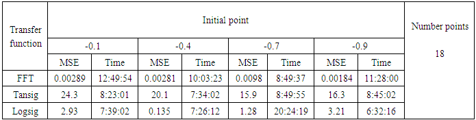
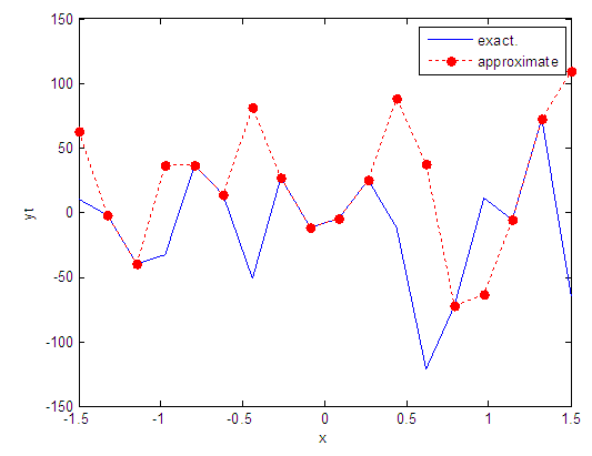
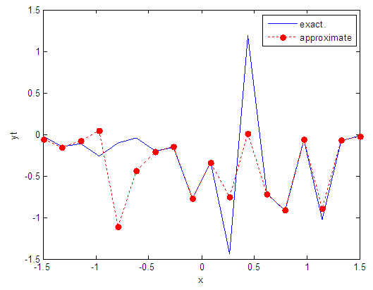
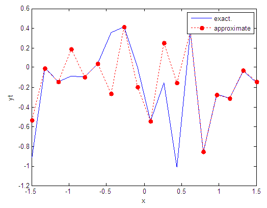
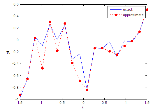
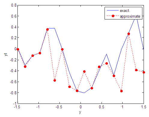
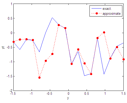
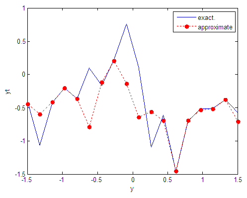
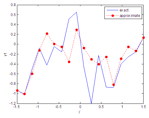
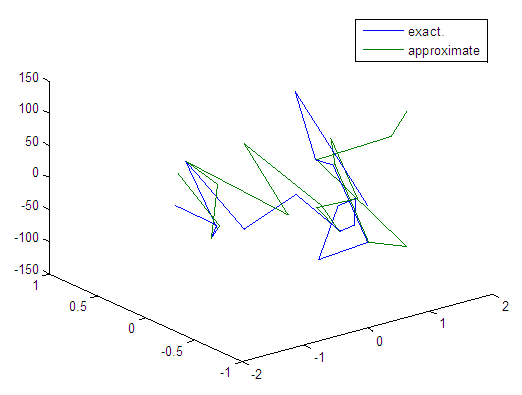
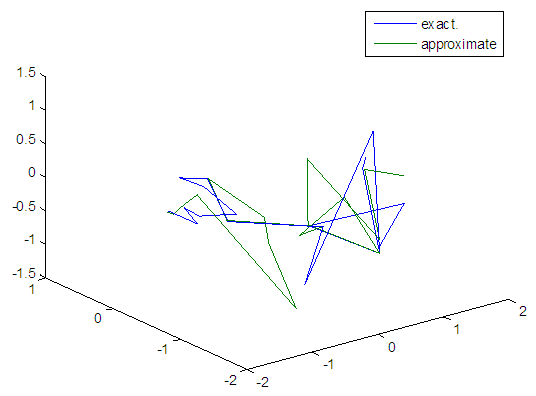
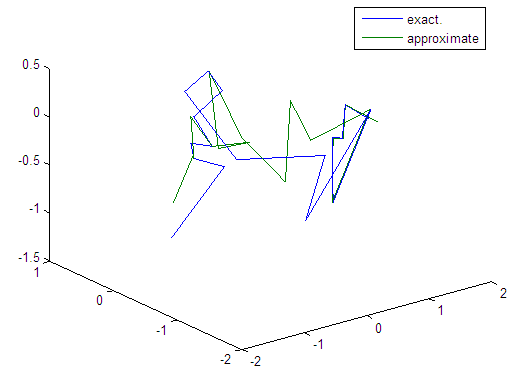
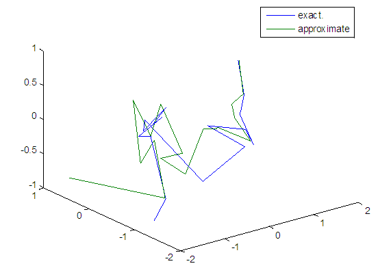
We will train the case when the Tinkerbell map is chaotic a=0.9, b= -0.6103, c=2 and d=0.5 and train the input data (x and y ) separately using the proposed FFNNs with one input, one output and tow hidden layers and we train this case with three types of transfer functions Tansig, logsig, and FFT.

Table (1) contains the results. Figures from (3) to (14) show the Real and approximate Tinkerbell dynamical map with different situations.

The weighted MSE is used as performance function according to x and y performance functions weights.

Table (1). Time and MSE of approximate solution after many training trials by using different transfer functions

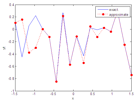
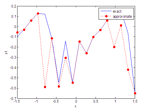Figure 3. Real and approximate Tinkerbell dynamical map with initial point x=-0.1 using FFT transfer function

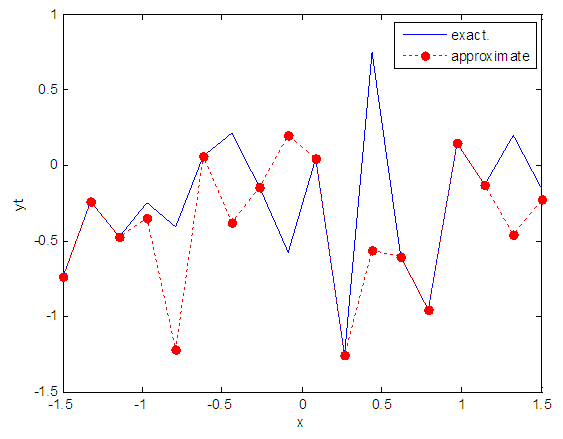
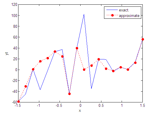
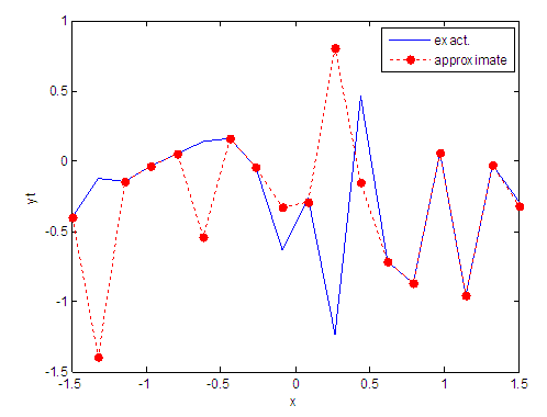Figure 4. Real and approximate Tinkerbell dynamical map with initial point x=-0.4 using FFT transfer function

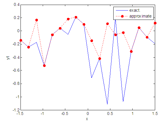
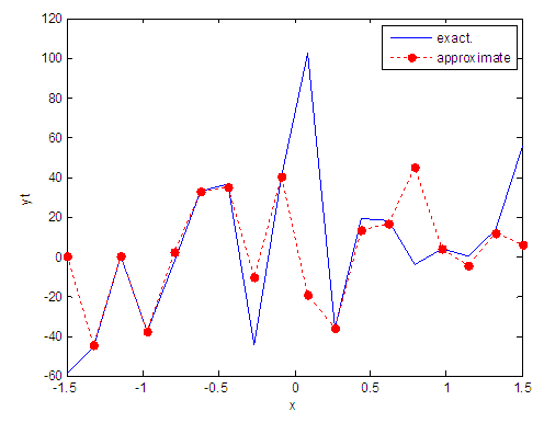
Figure 5. Real and approximate Tinkerbell dynamical map with initial point x=-0.7 using FFT transfer function

Figure 6. Real and approximate Tinkerbell dynamical map with initial point x=-0.9 using FFT transfer function

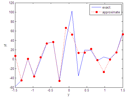
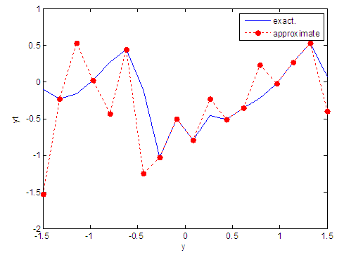Figure 7. Real and approximate Tinkerbell dynamical map with initial point y=-0.1 using FFT transfer function

Figure 8. Real and approximate Tinkerbell dynamical map with initial point y=-0.4 using FFT transfer function

Figure 9. Real and approximate Tinkerbell dynamical map with initial point y=-0.7 using FFT transfer function

Figure 10. Real and approximate Tinkerbell dynamical map with initial point y=-0.9 using FFT transfer function

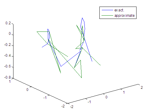Figure 11. Real and approximate Tinkerbell dynamical map with initial points x=-0.1 & y=-0.1 using FFT transfer function

Figure 12. Real and approximate Tinkerbell dynamical map with initial points x=-0.4 & y=-0.4 using FFT transfer function

Figure 13. Real and approximate Tinkerbell dynamical map with initial points x=-0.7 & y=-0.7 using FFT transfer function

Figure 14. Real and approximate Tinkerbell dynamical map with initial points x=-0.9 & y=-0.9 using FFT transfer function

4.1. Results Discussion

The experimental results from above table (1) show that the logsig, tansig and FFT transfer functions with proposed FFNN have a very good performance when the Tinkerbell map is chaotic. But the FFT transfer function is faster than logsig and tansig transfer functions to get results for all initial points.

5. Description of Training Process for Tinkerbell Map with Noise

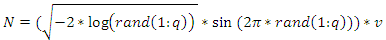
Here we train the normal and logistic noisy data of Tinkerbell map by using the suggested network with tansig, logsig and FFT transfer functions. It is suitable to choose the maximum number of epochs to reach high performance. It is worth to mention that the run size is k=1000.

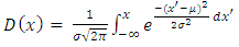
5.1. Normal Distribution [34]

Let x be a normally distributed random variable with mean and variance , where with probability density function and cumulative distribution function are respectively,

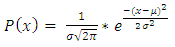(13)

(14)

One can generate values from Normal random variable as follows,

(15)

Where q is represents the number point and v is represent the variance.

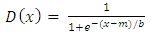
5.2. Logistic Distribution [34]

Let x be a Logistic distributed random variable with parameters and , where with probability density function and cumulative distribution function are respectively,

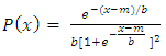(16)

(17)

One can generate values from Logistic random variable as follows,

(18)

Where q is represents the number point and v is represent the variance.

5.3. Training the Case with Normal Noise

The training process is conducted with variances 0.05, 0.5, 40 and 60.

Table (2) contains the results. Figures from (15) to (62) show the Real and approximate Tinkerbell dynamical map with different situation.

Table (2). Time and MSE of approximate solution after many training trials with normal noise by using different transfer functions when the variance equal to 0.05

Figure 15. Real and approximate Tinkerbell dynamical map with normal noise (v=0.05) and initial point x=-0.1 using FFT transfer function

Figure 16. Real and approximate Tinkerbell dynamical map with normal noise (v=0.05) and initial point x=-0.4 using FFT transfer function

Figure 17. Real and approximate Tinkerbell dynamical map with normal noise (v=0.05) and initial point x=-0.7 using FFT transfer function

Figure 18. Real and approximate Tinkerbell dynamical map with normal noise (v=0.05) and initial point x=-0.9 using FFT transfer function

Figure 19. Real and approximate Tinkerbell dynamical map with normal noise (v=0.05) and initial point y=-0.1 using FFT transfer function

Figure 20. Real and approximate Tinkerbell dynamical map with normal noise (v=0.05) and initial point y=-0.4 using FFT transfer function

Figure 21. Real and approximate Tinkerbell dynamical map with normal noise (v=0.05) and initial point y=-0.7 using FFT transfer function

Figure 22. Real and approximate Tinkerbell dynamical map with normal noise (v=0.05) and initial point y=-0.9 using FFT transfer function

Figure 23. Real and approximate Tinkerbell dynamical map with normal noise (v=0.05) and initial points x=-0.1 & y=-0.1 using FFT transfer function

Figure 24. Real and approximate Tinkerbell dynamical map with normal noise (v=0.05) and initial points x=-0.4 & y=-0.4 using FFT transfer function

Figure 25. Real and approximate Tinkerbell dynamical map with normal noise (v=0.05) and initial points x=-0.7 & y=-0.7 using FFT transfer function

Figure 26. Real and approximate Tinkerbell dynamical map with normal noise (v=0.05) and initial points x=-0.9 & y=-0.9 using FFT transfer function

Table (3). Time and MSE of approximate solution after many training trials with normalnoise by using different transfer functions when the variance equal to 0.5

Figure 27. Real and approximate Tinkerbell dynamical map with normal noise (v=0.5) and initial point x=-0.1 using FFT transfer function

Figure 28. Real and approximate Tinkerbell dynamical map with normal noise (v=0.5) and initial point x=-0.4 using FFT transfer function

Figure 29. Real and approximate Tinkerbell dynamical map with normal noise (v=0.5) and initial point x=-0.7 using FFT transfer function

Figure 30. Real and approximate Tinkerbell dynamical map with normal noise (v=0.5) and initial point x=-0.9 using FFT transfer function

Figure 31. Real and approximate Tinkerbell dynamical map with normal noise (v=0.5) and initial point y=-0.1 using FFT transfer function

Figure 32. Real and approximate Tinkerbell dynamical map with normal noise (v=0.5) and initial point y=-0.4 using FFT transfer function

Figure 33. Real and approximate Tinkerbell dynamical map with normal noise (v=0.5) and initial point y=-0.7 using FFT transfer function

Figure 34. Real and approximate Tinkerbell dynamical map with normal noise (v=0.5) and initial point y=-0.9 using FFT transfer function

Figure 35. Real and approximate Tinkerbell dynamical map with normal noise (v=0.5) and initial points x=-0.1 & y=-0.1 using FFT transfer function

Figure 36. Real and approximate Tinkerbell dynamical map with normal noise (v=0.5) and initial points x=-0.4 & y=-0.4 using FFT transfer function

Figure 37. Real and approximate Tinkerbell dynamical map with normal noise (v=0.5) and initial points x=-0.7 & y=-0.7 using FFT transfer function

Figure 38. Real and approximate Tinkerbell dynamical map with normal noise (v=0.5) and initial points x=-0.9 & y=-0.9 using FFT transfer function

Table (4). Time and MSE of approximate solution after many training trials with normal noise by using different transfer functions when the variance equal to 40

Figure 39. Real and approximate Tinkerbell dynamical map with normal noise (v=40) and initial point x=-0.1 using FFT transfer function

Figure 40. Real and approximate Tinkerbell dynamical map with normal noise (v=40) and initial point x=-0.4 using FFT transfer function

Figure 41. Real and approximate Tinkerbell dynamical map with normal noise (v=40) and initial point x=-0.7 using FFT transfer function

Figure 42. Real and approximate Tinkerbell dynamical map with normal noise (v=40) and initial point x=-0.9 using FFT transfer function

Figure 43. Real and approximate Tinkerbell dynamical map with normal noise (v=40) and initial point y=-0.1 using FFT transfer function

Figure 44. Real and approximate Tinkerbell dynamical map with normal noise (v=40) and initial point y=-0.4 using FFT transfer function

Figure 45. Real and approximate Tinkerbell dynamical map with normal noise (v=40) and initial point y=-0.7 using FFT transfer function

Figure 46. Real and approximate Tinkerbell dynamical map with normal noise (v=40) and initial point y=-0.9 using FFT transfer function

Figure 47. Real and approximate Tinkerbell dynamical map with normal noise (v=40) and initial points x=-0.1 & y=-0.1 using FFT transfer function

Figure 48. Real and approximate Tinkerbell dynamical map with normal noise (v=40) and initial points x=-0.4 & y=-0.4 using FFT transfer function

Figure 49. Real and approximate Tinkerbell dynamical map with normal noise (v=40) and initial points x=0.7 & y=0.7 using FFT transfer function

Figure 50. Real and approximate Tinkerbell dynamical map with normal noise (v=40) and initial points x=-0.9 & y=-0.9 using FFT transfer function

Table (5). Time and MSE of approximate solution after many training trials with normal noise by using different transfer functions when the variance equal to 60

Figure 51. Real and approximate Tinkerbell dynamical map with normal noise (v=60) and initial point x=-0.1 using FFT transfer function

Figure 52. Real and approximate Tinkerbell dynamical map with normal noise (v=60) and initial point x=-0.4 using FFT transfer function

Figure 53. Real and approximate Tinkerbell dynamical map with normal noise (v=60) and initial point x=-0.7 using FFT transfer function

Figure 54. Real and approximate Tinkerbell dynamical map with normal noise (v=60) and initial point x=-0.9 using FFT transfer function

Figure 55. Real and approximate Tinkerbell dynamical map with normal noise (v=60) and initial point y=-0.1 using FFT transfer function

Figure 56. Real and approximate Tinkerbell dynamical map with normal noise (v=60) and initial point y=-0.4 using FFT transfer function

Figure 57. Real and approximate Tinkerbell dynamical map with normal noise (v=60) and initial point y=-0.7 using FFT transfer function

Figure 58. Real and approximate Tinkerbell dynamical map with normal noise (v=60) and initial point y=-0.9 using FFT transfer function

Figure 59. Real and approximate Tinkerbell dynamical map with normal noise (v=60) and initial points x=-0.1 & y=-0.1 using FFT transfer function

Figure 60. Real and approximate Tinkerbell dynamical map with normal noise (v=60) and initial points x=-0.4 & y=-0.4 using FFT transfer function

Figure 61. Real and approximate Tinkerbell dynamical map with normal noise (v=60) and initial points x=-0.7 & y=-0.7 using FFT transfer function

Figure 62. Real and approximate Tinkerbell dynamical map with normal noise (v=60) and initial points x=-0.9 & y=-0.9 using FFT transfer function

5.4. Training with Logistic Noise

The training process is conducted with variances 0.05, 0.5, 40 and 60.

Tables from (6) to (9) contain the results. Figures from (63) to (110) show the Real and approximate Tinkerbell dynamical map with different situation.

Table (6). Time and MSE of approximate solution after many training trials with logistic noise by using different transfer functions when the variance equal to 0.05

Figure 63. Real and approximate Tinkerbell dynamical map with logistic noise (v=0.05) and initial point x=-0.1 using FFT transfer function

Figure 64. Real and approximate Tinkerbell dynamical map with logistic noise (v=0.05) and initial point x=-0.4 using FFT transfer function

Figure 65. Real and approximate Tinkerbell dynamical map with logistic noise (v=0.05) and initial point x=-0.7 using FFT transfer function

Figure 66. Real and approximate Tinkerbell dynamical map with logistic noise (v=0.05) and initial point x=-0.9 using FFT transfer function

Figure 67. Real and approximate Tinkerbell dynamical map with logistic noise (v=0.05) and initial point y=-0.1 using FFT transfer function

Figure 68. Real and approximate Tinkerbell dynamical map with logistic noise (v=0.05) and initial point y=-0.4 using FFT transfer function

Figure 69. Real and approximate Tinkerbell dynamical map with logistic noise (v=0.05) and initial point y=-0.7 using FFT transfer function

Figure 70. Real and approximate Tinkerbell dynamical map with logistic noise (v=0.05) and initial point y=-0.9 using FFT transfer function

Figure 71. Real and approximate Tinkerbell dynamical map with logistic noise (v=0.05) and initial points x=-0.1 & y=-0.1 using FFT transfer function

Figure 72. Real and approximate Tinkerbell dynamical map with logistic noise (v=0.05) and initial points x=-0.4 & y=-0.4 using FFT transfer function

Figure 73. Real and approximate Tinkerbell dynamical map with logistic noise (v=0.05) and initial points x=-0.7 & y=-0.7 using FFT transfer function

Figure 74. Real and approximate Tinkerbell dynamical map with logistic noise (v=0.05) and initial points x=-0.9 & y=-0.9 using FFT transfer function

Table (7). Time and MSE of approximate solution after many training trials with logistic noise by using different transfer functions when the variance equal to 0.5

Figure 75. Real and approximate Tinkerbell dynamical map with logistic noise (v=0.5) and initial point x=-0.1 using FFT transfer function

Figure 76. Real and approximate Tinkerbell dynamical map with logistic noise (v=0.5) and initial point x=-0.4 using FFT transfer function

Figure 77. Real and approximate Tinkerbell dynamical map with logistic noise (v=0.5) and initial point x=-0.7 using FFT transfer function

Figure 78. Real and approximate Tinkerbell dynamical map with logistic noise (v=0.5) and initial point x=-0.9 using FFT transfer function

Figure 79. Real and approximate Tinkerbell dynamical map with logistic noise (v=0.5) and initial point y=-0.1 using FFT transfer function

Figure 80. Real and approximate Tinkerbell dynamical map with logistic noise (v=0.5) and initial point y=-0.4 using FFT transfer function

Figure 81. Real and approximate Tinkerbell dynamical map with logistic noise (v=0.5) and initial point y=-0.7 using FFT transfer function

Figure 82. Real and approximate Tinkerbell dynamical map with logistic noise (v=0.5) and initial point y=-0.9 using FFT transfer function

Figure 83. Real and approximate Tinkerbell dynamical map with logistic noise (v=0.5) and initial points x=-0.1 & y=-0.1 using FFT transfer function

Figure 84. Real and approximate Tinkerbell dynamical map with logistic noise (v=0.5) and initial points x=-0.4 & y=-0.4 using FFT transfer function

Figure 85. Real and approximate Tinkerbell dynamical map with logistic noise (v=0.5) and initial points x=-0.7 & y=-0.7 using FFT transfer function

Figure 86. Real and approximate Tinkerbell dynamical map with logistic noise (v=0.5) and initial points x=-0.9 & y=-0.9 using FFT transfer function

Table (8). Time and MSE of approximate solution after many training trials with logistic noise by using different transfer functions when the variance equal to 40

Figure 87. Real and approximate Tinkerbell dynamical map with logistic noise (v=40) and initial point x=-0.1 using FFT transfer function

Figure 88. Real and approximate Tinkerbell dynamical map with logistic noise (v=40) and initial point x=-0.4 using FFT transfer function

Figure 89. Real and approximate Tinkerbell dynamical map with logistic noise (v=40) and initial point x=-0.7 using FFT transfer function

Figure 90. Real and approximate Tinkerbell dynamical map with logistic noise (v=40) and initial point x=-0.9 using FFT transfer function

Figure 91. Real and approximate Tinkerbell dynamical map with logistic noise (v=40) and initial point y=-0.1 using FFT transfer function

Figure 92. Real and approximate Tinkerbell dynamical map with logistic noise (v=40) and initial point y=-0.4 using FFT transfer function

Figure 93. Real and approximate Tinkerbell dynamical map with logistic noise (v=40) and initial point y=-0.7 using FFT transfer function

Figure 94. Real and approximate Tinkerbell dynamical map with logistic noise (v=40) and initial point y=-0.9 using FFT transfer function

Figure 95. Real and approximate Tinkerbell dynamical map with logistic noise (v=40) and initial points x=-0.1 & y=-0.1 using FFT transfer function

Figure 96. Real and approximate Tinkerbell dynamical map with logistic noise (v=40) and initial points x=-0.4 & y=-0.4 using FFT transfer function

Figure 97. Real and approximate Tinkerbell dynamical map with logistic noise (v=40) and initial points x=-0.7 & y=-0.7 using FFT transfer function

Figure 98. Real and approximate Tinkerbell dynamical map with logistic noise (v=40) and initial points x=-0.9 & y=-0.9 using FFT transfer function

Table (9). Time and MSE of approximate solution after many training trials with logistic noise by using different transfer functions when the variance equal to 60

Figure 99. Real and approximate Tinkerbell dynamical map with logistic noise (v=60) and initial point x=-0.1 using FFT transfer function

Figure 100. Real and approximate Tinkerbell dynamical map with logistic noise (v=60) and initial point x=-0.4 using FFT transfer function

Figure 101. Real and approximate Tinkerbell dynamical map with logistic noise (v=60) and initial point x=-0.7 using FFT transfer function

Figure 102. Real and approximate Tinkerbell dynamical map with logistic noise (v=60) and initial point x=-0.9 using FFT transfer function

Figure 103. Real and approximate Tinkerbell dynamical map with logistic noise (v=60) and initial point y=-0.1 using FFT transfer function

Figure 104. Real and approximate Tinkerbell dynamical map with logistic noise (v=60) and initial point y=-0.4 using FFT transfer function

Figure 105. Real and approximate Tinkerbell dynamical map with logistic noise (v=60) and initial point y=-0.7 using FFT transfer function

Figure 106. Real and approximate Tinkerbell dynamical map with logistic noise (v=60) and initial point y=-0.9 using FFT transfer function

Figure 107. Real and approximate Tinkerbell dynamical map with logistic noise (v=60) and initial points x=-0.1 & y=-0.1 using FFT transfer function

Figure 108. Real and approximate Tinkerbell dynamical map with logistic noise (v=60) and initial points x=-0.4 & y=-0.4 using FFT transfer function

Figure 109. Real and approximate Tinkerbell dynamical map with logistic noise (v=60) and initial points x=-0.7 & y=-0.7 using FFT transfer function

Figure 110. Real and approximate Tinkerbell dynamical map with logistic noise (v=60) and initial points x=-0.9 & y=-0.9 using FFT transfer function

5.5. Results Discussion

The two dimension Tinkerbell with noise normal and logistic, we see that the results of logsig transfer function when the variance (0.05 and 0.5), results of tansig transfer function and the results FFT in tables (2, 3, 6 and 7) are near in Performance and time. When the variance is increased to be 40 and 60, we need more time to get a good performance sometimes up to Hours. The performance FFT transfer functions is better than other transfer Functions see tables (4, 5, 8 and 9).

6. Summary

From the above cases, it is clear that the suggestion of FFT as transfer function in artificial neural network gives excellent results and good accuracy with and without noise in compare with traditional transfer functions (see Tables (1) – (9) ) for two dimension dynamical map (Tinkerbell). Therefore, we can conclude that the FFNN with FFT as transfer function which we proposed can handle effectively on the two dimension dynamical maps and provide accurate approximate solution throughout the whole domain and not only at the training set. As well, one can use the interpolation techniques to find the approximate solution at points between the training points or at points outside the training set. The estimation of Tinkerbell dynamical map obtained by trained Ann's offer some advantages, such as:

1. Complexity of computations increases with the increase of the number of sampling points in Tinkerbell dynamical map.

2. The FFNNs with FFT transfer function provides a solution with very good performance function in compare with other traditional transfer functions

3. The proposed FFNNs with FFT transfer function can be applied to two dimension dynamical maps

4. The proposed transfer function FFT gave best rustles especially when the Tinkerbell dynamical map is chaotic and noisy chaotic.

5. In general, the experimental results show that the FFNN side by side FFT transfer function which proposed can handle effectively Tinkerbell dynamical map and provide accurate approximate solution throughout the whole domain, because three points the first point neural network computations is parallel the second point FFT analysis of data and computations are parallel and third point FFT transfer function returns differences in data to sources original related homogeneity data and sectors of the work.

Some future works can be recommended. These works is as follows

1. Using networks with three or more hidden layers.

2. Using the architecture feedback neural network.

3. Increase the neurons in each hidden layer.

4. Use anther random variables as noise on Tinkerbell dynamical map.

5. Choose initial weights to be distributed as different random variables.

6. We recommended using FFT as transfer function in practical application.