Md Shakhawat Hossain
Department of Statistics, University of Chittagong, Chittagong, Bangladesh
Correspondence to: Md Shakhawat Hossain, Department of Statistics, University of Chittagong, Chittagong, Bangladesh.
| Email: |  |
Copyright © 2019 The Author(s). Published by Scientific & Academic Publishing.
This work is licensed under the Creative Commons Attribution International License (CC BY).
http://creativecommons.org/licenses/by/4.0/

Abstract
The aim of this study is to discuss the weakness of the conventional way of presenting the relative intensities in multiplicative models. The identification problem in hazards models with multiple interactions is illustrated here. A proposed solution of this problem with a common baseline level rather than of using two pairs of baseline levels is demonstrated. A Bayesian approach with Markov Chain Monte Carlo (MCMC) algorithm is used to estimate the parameters of interest of a hazards model with multiple interactions. In this analysis MCMC chain has run for 12000 iterations then first 2000 are discarded as burn-in and retained 10000 for the posterior distribution. Various diagnostics like posterior autocorrelations, Gelman-Rubin diagnostic, Monte Carlo Standard Error (MCSE) are performed to check the Markov chain mixing and convergence to target posterior distribution. All these diagnostics are found statistically significant. The results are presented in a single table with common baseline level according to proposed solution. The major consequences of such presentation is that it is almost impossible to compare two separate tables entirely, while from a single table one can easily compare and interpret the results properly. Relative intensities are also computed from the posterior simulations in Bayesian analysis and presented in different tables and graphs.
Keywords:
Hazards Model, Identification Problem, Relative Intensities, MCMC algorithm
Cite this paper: Md Shakhawat Hossain, A Bayesian Approach to Exemplify the Identification Problem in Discrete-time Hazards Models with Multiple Interactions, Applied Mathematics, Vol. 9 No. 1, 2019, pp. 13-23. doi: 10.5923/j.am.20190901.03.
1. Introduction and Literature Review
Presentation of results of any research work should be apparent so that one can easily understand and compare these. Especially it is more important in case of presenting relative intensities (risk) in models with multiple interactions. The identification problem in a hazards model with multiple interactions has been illustrated using a real data set.Hazards models, also known as duration or survival models, are widely used in different fields. They are used to analyze factors associated with the occurrence and timing of events such as finding a job, or dying. Cox introduced the proportional hazards model in which the covariates act in a multiplicative way on a baseline hazards function such that the hazards functions are proportional to each other over time for different values of the covariates [1]. This model has gained much popularity because no assumption is required on the form of the hazards function. Multiplicative model leads to a relative-risk type summary. Bernhardt and Bjeren used a multiplicative intensity model to investigate sex-differentials of first-birth to cohabiting and married Swedish adults [2]. The model controls for five socio-demographic variables-Sex, Education, Residence, Age, and Duration. In their final analysis, the authors found a five-factor two-interaction model that fits the data best.Scheike and Zhang proposed an additive-multiplicative intensity model that extended the Cox regression model as well as the additive Aalen model [3]. Instead of having simple baseline intensity the extended model used an additive Aalen model as its covariate dependent baseline. Approximate maximum likelihood estimators of the baseline intensity functions and the relative risk parameters of the Cox model are suggested by solving the score equations. Woodworth and Kanane used a discrete-time proportional hazards model of time to involuntary employment termination [4]. With this model they examined both continuous effect of the age of an employee and whether that effect has varied over time. Ghilagaber examined a multiplicative intensity model in which a covariate interacts with two other covariates in the same model [5]. He also demonstrated that the usual presentations of results of fitted model are miss specified approach and this approach provide less than interaction. In his paper the author suggested how the model can be given a mathematical representation applying the log-linear parameterization and also demonstrated that in saturations where a covariate interacts with two others to multiplicative model. Finally he showed the appropriate tables one should use to convey the empirical results. But he did not have original data in his hand and hence failed to re-analyze, he just used the results of Bernhardt and Bjeren [2]. Susarla and Van Ryzin have derived a nonparametric Bayesian estimator (NPBE) of the survival function for right-censored data for the first time [6]. Their estimator is based on the class of Dirichlet processes a priori introduced by Ferguson [7]. They proved that the nonparametric Bayesian estimator includes the Kaplan-Meier estimator as a special case, both estimators are asymptotically equivalent and that NPBE has better small sample properties than the Kaplan-Meier estimator [8]. Chong et al. have developed a Bayesian approach of model fitting to estimate age-specific survival rates for nesting studies using a large class of prior distributions [9]. The computation is done by Gibbs sampling and some latent variables are introduced to simply the full conditional distributions. Their results indicated that Bayesian analysis provides stable and accurate estimates of nest survival rate. Wong et al. used Bayesian approach to analyze a set of multilevel clustered interval-censored data from a clinical study to investigate the effectiveness of silver diamine fluoride and sodium fluoride varnish in arresting active dentin caries in Chinese pre-school children [10].There are a few researches have been done yet about the aforementioned problem of identification in multiplicative hazards models with a real data set. In addition a Bayesian approach is applied to fit a hazards model with multiple interactions for grouped survival data.The outline of this paper is as follows. In section 2, data and methodology is discussed. Results and discussion is described in section 3. Finally limitations and conclusion are presented in sections 4 and 5 respectively.
2. Data and Methodology
2.1. Source of Data
This study has utilized the data refers to childhood mortality among 7055 Eritrean children born in the period 2001 to 2010. This data is extracted from the Eritrea Demographic and Health Survey (EDHS) which was conducted in the period 2001 to 2010 by the National Statistics Office [Eritrea] and Macro International Inc. [11]. The EDHS employed a nationally representative, two-stage probability sample. In the first stage, 208 primary sampling units (PSUs) were selected with probability proportional to size. A complete listing of the households in the selected PSUs was carried out. The lists of households obtained were used as the frame for the second-stage sampling, which was the selection of the households to be visited by the EDHS interviewing teams during the main survey fieldwork. Women between the ages of 15 and 49 were identified in these households and interviewed. A total of 6258 households were selected in the sample, of which 5642 were occupied at the time of the survey. In the interviewed households 5250 eligible women identified of whom 5054 were interviewed, yielding a response rate of 96 percent. The information related to early childhood mortality drawn from the questions asked in the birth history section of the women’s questionnaire. In the birth history, for each live birth, information is collected on sex, month and year of birth, survivorship status and current age, and age at death if the child died. The study consists of the following variables:ExpMonth is the exposure time (in months) i.e. the number of months between child’s birth and interview time (if the child was alive) or age in months at the time of death (if the child has died). Occurrence indicates the number child died in the time between birth and date of interview. It is measured form the Status which is an indicator of whether the child still survives (Status = 0), or died (Status = 1). Period indicates the child’s period of birth (birth cohort) and takes value 1 for the period 2001-05 and 2 for the period 2006-10. Mother’s Education indicates mother’s educational level and has value 1 if she has no education at all, 2 if she had primary-level education, 3 if her educational level is secondary-level or above. Residence has value 1 for urban areas and 2 for rural areas.The time variable (ExpMonth) is partitioned into 4 age-groups such that age_g1 covers the period 1-11 months, age_g2 covers the period 12-23 months, age_g3 covers the period 24-35 months, and age_g4 covers the period 36-59 months.
2.2. Parameter Estimation of Multiplicative Hazards Model for Grouped Data
For the present study of illustrating the identification problem in hazards models, the one important issue is variation across individuals within the population rather than the functional form between time and the rate. In this section, therefore, we shall concentrate on the piecewise exponential model in which the hazards rate remains constant within certain time interval but varies arbitrarily among the intervals. Let Dij denote the number of occurrences (say deaths) of the event of interest in the i-th time (discrete/grouped) interval and j-th level of the covariate, for Tij time units (say, months) of exposure to the risk of experiencing the event. We interpret each occurrence or exposure rate  as an estimator of the corresponding hazards function
  which, as in the piecewise exponential model, is assumed to be constant at each combination (i,j) of the levels. In other words, the density function of the time to occurrence of an event in duration interval i for a person with level j of the covariate is given by
 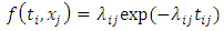 | (1) |
The rate variability across individuals in a population can be modeled by specifying the rate as a function of a set of explanatory variables. When all these variables are categorical, a simple mathematical model for the rate structure is given by  | (2) |
whereby the interval-specific hazards rates are obtained from multiplicative contributions of the i-th interval (θi) and j-th level of the covariate (αj). A model of this form has been suggested for a variety of situations.Equation (2) will be referred to as a multiplicative parameterization of the hazards (intensity) rate. θi is the baseline intensity (value of the intensity rate when αj=1), while αj represents the intensity of an individual with level j of the covariate relative to that of an individual with the baseline level j0. Let us define Ai= lnθi, and Bj=lnαj so that lnλij=lnθi+lnαj=Ai+Bj. If we further let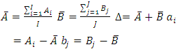 We may define a log-linear equivalent of the intensity rate in (2) as
  | (3) |
Thus one can estimate the intensity rates as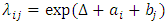 | (4) |
This is a log-linear parameterization of the intensity rate. Without the loss of generality, we may select j0 to be the first level (j0=1). Then, since by design α1=1, we have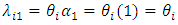 or, equivalently
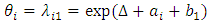 | (5) |
as the estimate of baseline intensity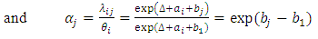 | (6) |
as the estimate of relative intensity.Details on procedures for estimating the parameters in (2) and/or (4) may be found in [12] and [13]. The extension with three factors indexed by i, j, and k, in which the first two factors interact, equations in (2) and (4) may be extended to  | (7) |
and  | (8) |
Further consider a multiplicative hazards rate model that factor age-group (i) interacts with the covariates period (j) and mother’s education (k) while residence (l) is not involved in any interaction. Thus the mathematical representation for this multiplicative hazards model as in (2) is  | (9) |
while the corresponding log-linear model is given by  | (10) |
or equivalently, | (11) |
where Δ = Intercept, ai = i-th age-group, bj= j-th period, ck= k-th mother’s education, dl= l-th residence, eij = Interaction between i-th age-group and j-the period, and fik = Interaction between i-th age-group and k-th mother’s education.Now the relative intensities for the interaction between age-group and period: | (12) |
Similarly the relative intensities for the interaction between age-group and mother’s education: | (13) |
2.3. The Identification Problem
Recall that the baseline intensity is given by [from equation (11)] | (14) |
Thus the model in (19) can be represented as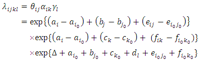 [From equations(12), (13) and (14)]
 | (15) |
This expression is different from that in (19) because it contains the additional term (ai-ai0) in the exponent. If we redefine  | (16) |
and for some unspecified 
 | (17) |
Then we get | (18) |
which is identical to in (11). The problem is to choose  ≠1. It is impossible to partition the contribution of (ai-ai0), in a unique way, among the two exponents in (16) and (17). In other words, the relative intensities
  and
and  become unidentified in the sense that they cannot be represented in a unique way.
2.4. Proposed Solution
A proposed solution for the aforementioned problem according to Ghilagaber (1999) is to use a common baseline level for all the factors involved in interactions rather than of using two pairs of baseline levels. Therefore the relative intensities of interest are computed using a common baseline level for the factors involved in interactions. Let  denotes the relative intensity at the i-th level of the covariate age-group, j-th level of the covariate period, and k-th level of the covariate mother’s education. Our multiplicative hazards (intensity) model will then be given by
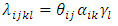 | (19) |
and the relative intensity of interest,  , is given by
 | (20) |
If we were to compute the joint effect of the three covariates involved in interaction using the mathematical representation in (20) and (21) with two pairs of baseline levels, such effect would have been obtained as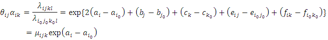 | (21) |
Thus | (22) |
which is different from the formulation in (19). In other words, it can be explained that the use of two pairs of baseline levels, instead of one common for the three factors involved in the interaction, will inflate the real intensity rate by a factor of  .Therefore in our multiplicative hazards model, the inflation factor of real intensity rate is given by
 | (23) |
Let us now re-estimate the relative intensities of interest using a common baseline levels for factors involved in interaction. The relative risks for the non-interacting factor residence and those of the baseline intensities remain unchanged.For the factors involved in interaction, we get the  table of relative intensities,
  , can obtain by
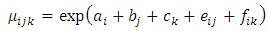 | (24) |
Further, we can compute the following relative intensities of interest:Age-group profiles of relative intensities across period: | (25) |
Age-group profiles of relative intensities across mother’s education: | (26) |
2.5. Bayesian Approach
Bayesian analysis is applied to estimate parameters of interest in multiplicative hazards model in (9) and compute relative intensities. The data, used in this study, is a grouped data of childhood mortality and thus it is a grouped survival data which are usually censored. Bayesian analysis in grouped data is widely used because of the direct probabilistic interpretation of the posterior distribution and because many problems can be formulated in terms of integrals with respect to the posterior distribution. The Bayesian approach delivers the answer to the right question in the sense that Bayesian inference provides answers conditional on the observed data and not based on the distribution of estimators or test statistics over imaginary samples not observed [14]. Bayesian inference is consistent with much of philosophy of science regarding epistemology, where knowledge cannot be built entirely through experimentation, but requires prior knowledge [15)]. The development of new numerical algorithms, such as Markov Chain Monte Carlo(MCMC) algorithm, which allow us to obtain a sample from the posterior of interest, has open the door to the use of Bayesian methods to survival analysis. In this study we use Bayesian approach with MCMC algorithm is used to estimate the parameters of interest of a hazards model with multiple interactions.MCMC method is a general simulation method for sampling from posterior distributions and computing posterior parameters of interest. In MCMC method samples are taken successively from a target distribution. Each sample depends on the previous one, hence the notion of the Markov chain. A Markov chain is a sequence of random variables,  , for which the random variable
  depends on all previous
  only through its immediate predecessor
  . With the MCMC method, it is possible to generate samples from an arbitrary posterior density
  and to use these samples to approximate expectations of quantities of interest. Most importantly, if the simulation algorithm is implemented correctly, the Markov chain is guaranteed to converge to the target distribution
  under rather broad conditions, regardless of where the chain was initialized. The usual programming statements for survival estimation are not directly applicable. Thomas and Reyes offered a tutorial in survival estimation for the time-varying coefficient model, implemented in SAS and R [16]. Allison presents a highly readable introduction to the subject based with Bayesian approach on the SAS statistical package, but nevertheless of general interest [17]. Statistical Analysis System (SAS) is used to analyze the data.
3. Results and Discussion
3.1. Fitting a Multiplicative Hazards Model Using Bayesian MCMC Algorithm
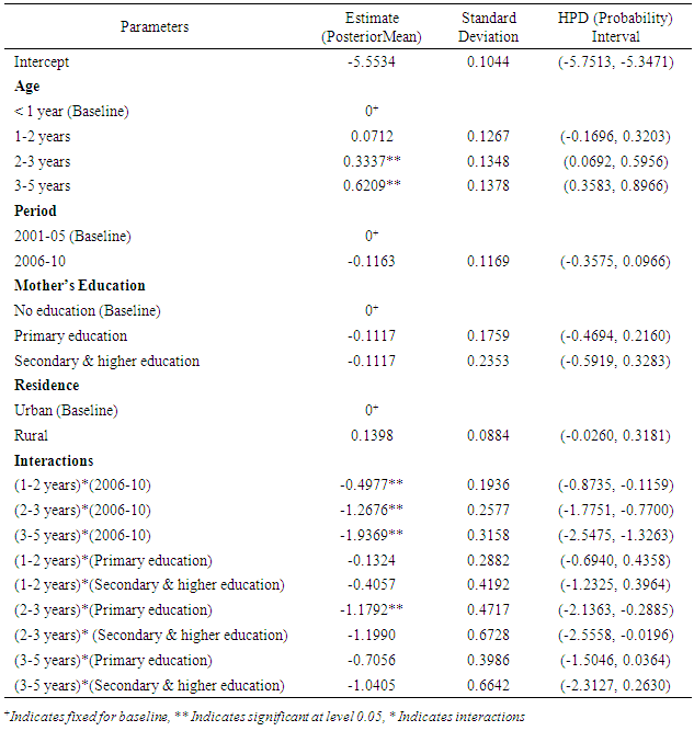
To fit a hazards model with multiple interactions in (9), we estimate the parameters of corresponding log-linear model in (10) applying Bayesian procedure for non-informative prior. In this model, samplings from the joint posterior distribution of the unknown quantities of interest are obtained through the use of MCMC methods. In this analysis MCMC chain is run for 12000 iterations, and then first 2000 are discarded as burn-in and retained 10000 for posterior analysis. The estimates (posterior mean) of parameters, Standard deviation and highest posterior density (HPD) intervals are given in the Table 1.The highest posterior density (HPD) intervals, also known as probability intervals or credible intervals, actually have the stated probability of containing the true value of the variable of interest. A 95% credible interval says simply that there is a probability of 0.95 that the true parameter is included in the reported interval. A 95% credible interval that does not include 0 is the Bayesian equivalent of an estimate that is significantly different from 0 at the .05 level (by a two-sided test). From the Bayesian HPD intervals in Table 1 it is observed that six estimates marked by double asterisk are statistically significant at 5% level of significance.Table 1. Bayesian estimate of parameters of interest in the log-linear model in (10)
 |
| |
|
Before drawing inferences from the posterior estimates and/or posterior simulations, we examined the trace, autocorrelation, density plots for each parameter are given in Appendix, and other related diagnostics to be content that the underlying chain has converged.
3.2. Some Diagnostics
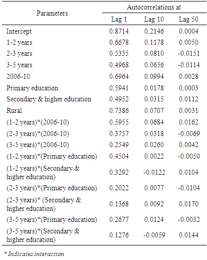
Posterior Autocorrelations: In this analysis it is sighted that the autocorrelations given in Table 2 can vary substantially among different lags and decline dramatically and at fifty draws apart (lag 50) close to 0 which suggests that the Markov chain is well mixing. Usually the well mixing chain produces better estimates of the parameters.Table 2. Posterior Autocorrelations with non-informative prior
 |
| |
|
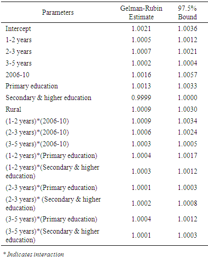
Gelman-Rubin diagnostics: The Gelman-Rubin estimates shown in the Table 3 are very close to 1.0 which indicating no evidence of a failure to converge.Table 3. Gelman-Rubin Diagnostics
 |
| |
|
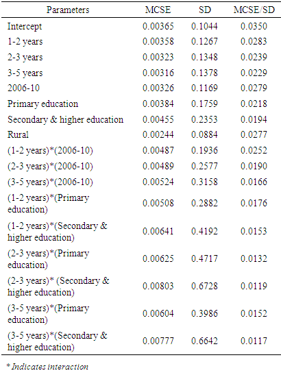
Monte Carlo Standard Errors: Table 4 shows the Monte Carlo Standard Error (MCSE), the posterior sample standard deviation (SD), and the ratio of the two reveal that the standard errors of the mean estimates for each of the parameters are relatively small, with respect to the posterior standard deviations. The ratios are also small, which imply that only a small fraction of the posterior variability is due to the simulation.Table 4. Monte Carlo Standard Errors
 |
| |
|
Again the trace plots of samples versus the simulation index (estimate), given in appendix, show excellent mixing, the autocorrelation decreases to near zero, and the density is bell-shaped. The trace plots are centered near their respective posterior mean and traverse the posterior space with small fluctuations suggesting that the chain has converged to its stationary distribution. For the intercept, the trace plot is centered near the posterior mean of -5.77. Samples in both tails are covered. These results exhibit convergence of the Markov chain to its stationary distribution.
3.3. Computation of Inflation Factor from Posterior Draws
The inflation factors of intensity rate for different levels of age-group (relative to age <1 year) are estimated from 10000 posterior draws using equation in (23). We compute 10000 estimates of inflation factors for each level of age-group and consider their mean as corresponding estimate and plot these 10000 computed values of inflation factors of intensity rate in Figure 1.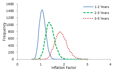 | Figure 1. Curves of inflation factors of intensity rate for different levels of age groups relative of age <1 year |
The estimates of inflation factor of intensity rate for different levels of age-group (relative to age <1 year) computed from posterior draws are 1.0824, 1.4088, and 1.8783 for ages 1-2 years, 2-3 years, and 3-5 years respectively. These quantities imply that the estimated intensities (relative to age <1 year) are inflated by factors 1.0824, 1.4088, and 1.8783 for ages 1-2 years, 2-3 years, and 3-5 years respectively when two pairs of baseline levels are used.Figure 1 shows that the curves are bell-shaped and peaked at their corresponding estimates stated above with small variability.
3.4. Computation of Relative Intensities of Interest from Posterior Draws
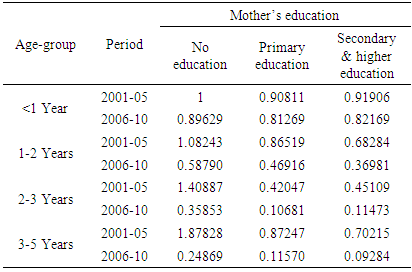
The relative intensities of interest with a common baseline level according to suggested solution are computed using equation (24) for age-group, period and mother’s education from the obtained 10000 posterior simulations of each estimate. We take the means of 10000 computed values of corresponding relative intensities for each estimate and are given in Table 5. Table 5. Relative intensities (μijk) with a common baseline level for age-group, period and mother’s education as in Table 4 calculated from posterior simulation
 |
| |
|
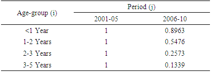
Table 5 represents the relative intensities considered in multiplicative hazards model with a common baseline level for covariates involved in interactions according to proposed solution. One can easily interpret and compare these relative intensities with different levels of covariates using the common baseline level from this single table. Further we compute relative intensities of age-group profiles across period from the 10000 posterior simulations of each estimate using equation (25) and take their means as corresponding estimates presented in Table 6. We also plot these 10000 calculated values for each relative intensity estimate in the same graph in Figure 2.Table 6. Age-group profiles of relative intensities across period calculated from posterior simulation
 |
| |
|
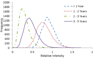
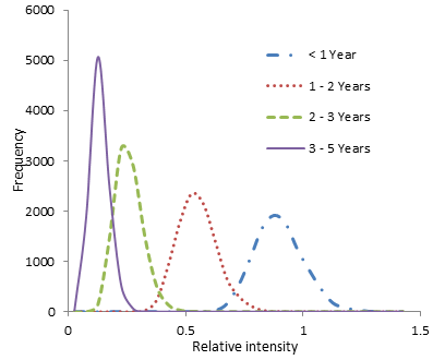 | Figure 2. Curves of 10000 estimates of relative intensities of child mortality for age groups across period 2006-10 compare to the period 2001-05 |
From Table 6 it is observed that children born in the period 2006-10 are less likely to death for all age groups as compared to the children having birth in 2001-05.In Figure 2 all the curves are bell-shaped and peaked around their corresponding mean estimates (0.89, 0.55, 0.26, and 0.13). Among these, the curves for age 2-3 years and 3-5 years across period 2006-10 are tidier compare to others, and indicate that these estimates have smaller variability. Figure 2 shows that the risk of child mortality is lower (estimates are less than 1) in the period 2006-2010 compare to the period 2001-2005 for all age groups and risk of child mortality gradually goes down with the increase of age which also conferred by the values in Table 6.Figure 3 shows that the risk of child mortality in rural area is higher (estimate is greater than 1) compare to that of in urban area. The curve is also so trim indicating estimate has small variability. 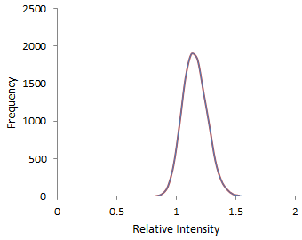 | Figure 3. Curves of 10000 estimates of relative intensities or risk of child mortality living in rural area compare to that in urban area |
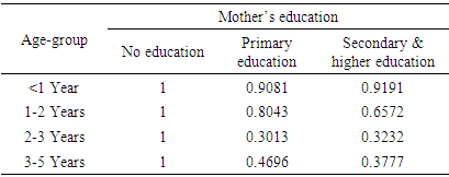
We also compute relative intensities of age-group profiles across mother’s education from the posterior simulations of estimates using equation (26) and are shown in Table 7. The calculated values from posterior simulations for corresponding estimate of relative intensities are plotted in Figure 4 and 5.Table 7. Age-group profiles of relative intensities across mother’s education calculated from posterior simulation
 |
| |
|
 | Figure 4. Curves of 10000 estimates of relative intensities of child mortality for age group across mother’s education primary level compare to mother’s have no education |
From Figure 4 it is observed that all the curves are bell-shaped and peaked around their corresponding estimates. Figure 4 also shows that the risk of child mortality for whose mother’s have primary education is lower (estimates are less than 1) than that of whose mother’s have no education for all age groups which conferred by the values of 3rd column in Table 7.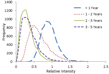 | Figure 5. Curves of 10000 estimates of relative intensities of child mortality for age group across mother’s education secondary level and higher compare to mother’s have no education |
Figure 5 shows that the risk of child mortality for whose mother’s have secondary and higher education is lower (estimates are less than 1) than that of whose mother’s have no education for all age groups which also conferred by the values of 4th column in Table 7.
4. Limitations
One of the limitations in this study is that we have used an old data set that is for the year 2001-2010. Since our main intension is to illustrate the identification problem of relative risk with a real data set i.e. this is a methodological study and hence this limitation would not be affected on our goal. Another limitation is in Bayesian analysis we have used non-informative prior due to lack of informative prior.
5. Conclusions
In this work the close relationship among the parameterizations in multiplicative hazards models is discussed. One such situation is arisen when a multiplicative hazards model involves a factor that interacts with two others in the same model. It is illustrated that, in such situations, the traditional approach of using a model with more than one baseline levels suffers from drawbacks. Consequently it is impossible to transform the intensity rate from log-linear parameterization into the simpler relative intensities format because the relative intensities related to the interacting factors are unidentified in the sense that they cannot be expressed in a unique way. To demonstrate the issues discussed, a real data set is used. It is revealed that using of two pairs of baseline levels might lead to estimates of relative intensities that inflated by a factor which is a function of the effects of the covariate interacting with the two other covariates. Moreover, the results are difficult to interpret. Thus a proposed solution is discussed that use a common baseline level for the factors involved in interaction and computed the relative intensities of interest.A hazards model with multiple interactions is fitted using Bayesian MCMC algorithm for non-informative prior. Different diagnostics and tests are performed to check the Markov chain mixing, convergence to target posterior distribution, and posterior variability. All these diagnostics and tests are found statistically significant. The trace plots of samples against the estimates obtained from MCMC simulations also showed excellent mixing, the autocorrelation decreases to near zero, and the density is bell-shaped. The trace plots are centered near their respective posterior mean with small fluctuations suggesting that the chain has converged to its same stationary distribution. In the proposed solution with common baseline level, the results are presented in a single table rather than two separate tables with two baseline levels. Some extra information can be extracted from the single table with common baseline level but not possible from conventional presentation. The main consequences is that it is almost impossible to compare the two separate tables entirely, while from a single table it is easy to compare and interpret results for anyone. Relative intensities are computed according to the proposed solution from the posterior simulations obtained in Bayesian analysis. It also plotted the computed 10000 values from posterior draws for each estimate. These graphs facilitate us to study the characteristics and distribution pattern of estimates.These ideas, methodologies, and results of the present study could be an inspiration to the researchers for further research in these areas.
ACKNOWLEDGEMENTS
I am very grateful to Dr. Gebrenegus Chilagaber, Professor, Department of Statistics, Stockholm University, Sweden for his extensive co-operation to do this piece of work. I would like to take this opportunity to thank all of my colleagues and staffs.
Appendix
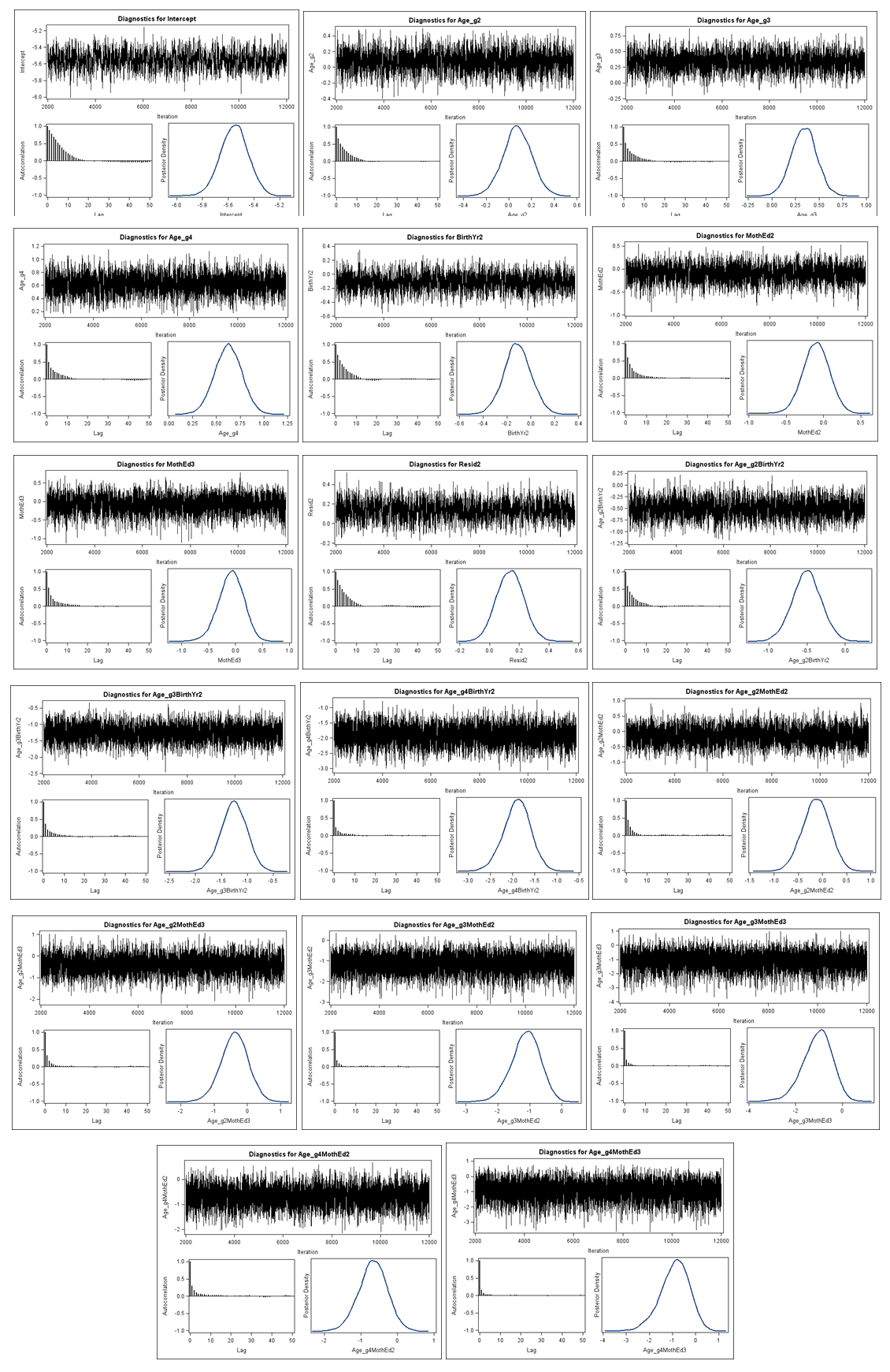 | Trace plots of samples versus the simulation index (estimate) in posterior draws: |
References
| [1] | Cox, D.R. (1972). Regression Models and Life Tables. Journal of the Royal Statistical Society B, 34(2): 187-220. |
| [2] | Bernhardt, E.M. and Bjeren, G. (1990). Quantitative Life History Analysis with Small Data Sets: A Study of Gender Differences in the Transition to Parenthood in Sweden. Paper Presented at the World Congress of Sociology, Madrid-Spain, July, 9-13. |
| [3] | Scheike, T.H. and Zhang, M.J. (2002). An Additive-Multiplicative Cox-Aalen Regression Model. Scandinavian Journal of Statistics, 29:75-88. |
| [4] | Woodworth, G. and Kanane, J. (2010). Age- and Time-varying Proportional Hazards Models for Employment Discrimination. The Annals of Applied Statistics, 4(3): 1139-1157. |
| [5] | Ghilagaber, G. (1999). On the Problem of Identification in Multiplicative Intensity-Rate Models with Multiple Interactions. Quality & Quantity, 33: 45-58. |
| [6] | Susarla, V. and Van Ryzin, J. (1976). Nonparametric Bayesian Estimatin of Survival Curves from Incomplete Observations. Journal of the American Statistical Association 71: 897-902. |
| [7] | Ferguson, T.S. (1973). A Bayesian Analysis of Some Nonparametric Problems. Annals of Statistics, 1:209-230. |
| [8] | Rai, K., Susarla, V. and Van Ryzin, J. (1980). Shrinkage Estimation in Nonparametric Bayesian Survival Analysis: A Simulation Study. Communications in Statics: Simulation and Computations, 3:271-298. |
| [9] | Chong, Z., Dongchu, S., and Yolande, T. (2001). Bayesian Modeling of Age-Specific Survival in Nesting Studies Under Dirichlet Priors, Biometrics, 57:1059-1066. |
| [10] | Wong, M.C.M., Lam, K.F., and Lo, E.C.M. (2005). Bayesian Analysis of Clustered Interval-censored Data. Journal of Dental Research 84(9): 817-821. |
| [11] | National Statistics Office [Eritrea] and Macro International Inc. (2010). Eritrea Demographic and Health Survey, 2010. Calverton, Maryland: National Statistics Office and Macro International Inc. |
| [12] | Laird, N. and Olivier, D. (1981). Covariance analysis of censored survival data usinglog-linear analysis technique. Journal of American Statistical Association, 76:231-240. |
| [13] | Ghilagaber, G. (1998). Analysis of Survival Data with Multiple Causes of Failure: A Comparison of Hazard-and Logistic-Regression Models with Application in Demography. Quality & Quantity, 32: 297-324. |
| [14] | Rossi, P., Allenby, G., and McCulloch, R. (2005). Bayesian Statistics and Marketing. John Wiley & Sons, West Sussex, England. |
| [15] | Roberts, C. (2007). The Bayesian Choice, 2nd edition. Springer, Paris, France. |
| [16] | Thomas, L. and Reyes, E.M. (2014). Tutorial: Survival Estimation for Cox Regression Models with Time-Varying Coefficients Using SAS. Journal of Statistical Software, 61:1-23. |
| [17] | Allison, P.D. (2010). Survival Analysis Using SAS: A Practical Guide, 2nd Edition. Cary, NC:SAS Institute Inc. |

 Abstract
 Reference
 Full-Text PDF
 Full-text HTML