Fatma D. M. Abdallah
Department of Animal Wealth Development, Faculty of Veterinary Medicine, Zagazig University, Egypt
Correspondence to: Fatma D. M. Abdallah, Department of Animal Wealth Development, Faculty of Veterinary Medicine, Zagazig University, Egypt.
| Email: |  |
Copyright © 2019 The Author(s). Published by Scientific & Academic Publishing.
This work is licensed under the Creative Commons Attribution International License (CC BY).
http://creativecommons.org/licenses/by/4.0/

Abstract
The goal of this study is to show the role of time series models in predicting process and to demonstrate the suitable type of it according to the data under study. Autoregressive integrated moving averages (ARIMA) model is used as a common and a more applicable model. Univariate ARIMA model is used here to forecast egg production in some layers depending on daily data from the period of May to October 2018. Different criteria of the ARIMA model can be used to choose the suitable one such as the coefficient of determination (R2), mean absolute error (MAE), root mean square error (RMSE) and mean absolute relative percentage error (MARPE). Depending on these measures the autoregressive integrated moving average model with ordering (2,2,1) is considered the best model for forecasting process. The model fit statistics such as RMSE (331.520) which was low and the lowest BIC value (11.745) indicating that the model fit the data well. The high value of R2 (0.95) and MAPE (4.542) indicated a perfect forecasting model. Also, ARIMA model with ordering (1,2,2) is good in prediction process.
Keywords:
Time series, Forecasting, ARIMA model, Autocorrelation
Cite this paper: Fatma D. M. Abdallah, Role of Time Series Analysis in Forecasting Egg Production Depending on ARIMA Model, Applied Mathematics, Vol. 9 No. 1, 2019, pp. 1-5. doi: 10.5923/j.am.20190901.01.
1. Introduction
Forecasting is a process to predict some of the future events of a specified variable. It is an outcome of analysis of past or present data. It is widely applied in many fields as it has a major role in increasing profit [1]. Forecasting techniques classified into qualitative and quantitative methods.A time series is a set of observations collected over time. It aims to determine the behavior of the series, identify the important parameters and forecast the future values of the time series.There are many classical forecasting methods (such as exponential smoothing, regression and others) can be used for prediction process of time series data. These methods differ according to the data features, number of data and presence of autocorrelation [2]. [3] presented what is called autoregressive integrated moving averages methods (ARIMA) model to predict the future values of the time series data. The most frequently used ones are autoregressive moving average (ARMA), and autoregressive integrated moving average (ARIMA) [4]. The ARIMA method is a technique used for building a good predicting model of time series data. There are some advantages and disadvantages of the model. The advantages of the ARIMA model were: it is a suitable and proper method particularly incase of short term time series forecasting [5]. Another advantage, it can elevate the prediction accuracy while maintaining the parameters numbers to a minimum. The major disadvantages was difficulty in application compared to other models such as exponential smoothing methods to understand [6].The characters of ARIMA model are stationarity (mean value or variance are constant over time), and the coefficients and the residuals are independent and normally distributed [7]. If the model is non-stationary, first differences of the series can be made to produce a new time series of successive differences (Yt,Yt-1). If first differences do not achieve the stationarity, the second differences of the series are taken and log transformation of the series also can be applied.As it is known that, the ARIMA model is consisted of (p, d, q) where, p is the autoregressive parameters, d is the number of differencing passes and q is the moving average parameters.There are many examples of application this model in forecasting future production for many years such as [8] who predicted Indian egg production for seven years.
2. Material and Methods
2.1. Source of Data
The study was carried out using daily egg production data obtained over 6 months, from May to October. Data were obtained from a farm in Sharkia governorate. This farm contain 9000 birds of BabCock BV-300 white egg laying chickens breed. The birds were brought as newly-hatched chicks at the beginning of the cycle (December 31, 2017) till now. Firstly, birds fed on starter ration of broilers till 21 days of rearing. Then the ration and its components changed to fit egg production during the rearing period. As these layers are highly producers, ARIMA technique is a good model in predicting the future performance of this farm.
2.2. Statistical Model
For ARIMA model, there are four important steps should be put in consideration to apply it. These steps are identification, estimation, diagnostic checking and forecasting. Model parameters were estimated using the Statistical Package for Social Sciences (SPSS) package to fit the ARIMA models in predicting egg production [8].Identification step applied to achieve stationarity and to build a suitable model using autocorrelation (ACFs), partial autocorrelation (PACFs), and transformations (differencing and logging). Estimation or specification step estimate coefficients depending on least squares and likelihood techniques such as AIC, BIC likelihood which introduced by [9] and [10].  | (1) |
 | (2) |
Where k = p+q+1 (if model includes intercept) otherwise, k = p+q. p and q are the model orders. The model considered well if its AIC and SBIC value is low [11].Diagnostics step depending on examining the parameters significance using charts, statistics, ACFs and PACFs of residuals to determine the model fitting [12]. Non-significant parameters can be removed from the model.Forecasting step can be applied in prediction process after checking the model in the previous steps.There are many accuracy measures applied after model selection helping in choosing the best model as mentioned by [13]. These measures include root mean square error (RMSE), mean absolute error (MAE), mean absolute percentage error (MAPE), mean error (ME) and mean percentage error (MPE). These measures are explained in Table 1.Table 1. Forecasts Accuracy Measuring Methods
 |
| |
|
The Box-Jenkins method is a combination of the autoregressive and the moving average methods, it is known as ARIMA (Autoregressive Integrated Moving Average) method [5].Autoregressive process of order (p) is | (9) |
where Yt is value of the series at time t, Yt-1,Yt-2,…Yt-p are dependent on the past values of the variable at specific time points, ϕ0,ϕ1,ϕ2,…,ϕp are the regression intercept (coefficient) and εt is error part (not explained by model).Moving Average (MA) Process of order (q) | (10) |
Where Yt is the value of the series at time t, θ0, θ1, θ2, θq are the (weights) coefficients applied to εt−1, εt−2, εt−q previous forecast errors and εt is the residual error.The general form of ARIMA model of order (p, d, q) is  | (11) |
Autocorrelation and partial autocorrelation function.Autocorrelation is a measure of the internal correlation within a time series. It is a technique of detecting internal relationship between values in a time series. Autocorrelation measures linear relationship, in a similar way with normal correlation.The partial autocorrelation function (PACF) gives the partial association of a time series with its own lagged observations, adjusting for the observations of the time series at all shorter lags. It unlikes the autocorrelation function (no controlling for other lags).This function introduces an important role in analysis process. Its role is identifying the extent of the lag in an autoregressive model. Box–Jenkins approach introduced this function to model time series data. Plotting the partial autocorrelation functions is helpful in detecting the suitable lags p in ARIMA (p,d,q) model.
3. Results and Discussion
3.1. Identification of ARIMA Model
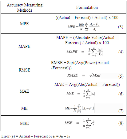
ARIMA model can be designed after achieving a stationarity (constant mean and constant variance) to the variable under forecasting by different transformation methods. Figure 1 showed that the pattern of the data under study were non-stationary and in this case transformation process (differencing and logging) of the data is used to become stationary data as shown in Figure 2.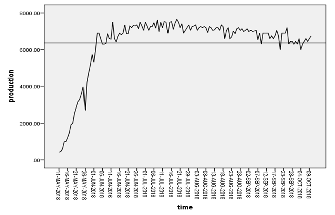 | Figure 1. Time series plot of egg production of the farm under study |
 | Figure 2. Time series plot of egg production (stationary data) |
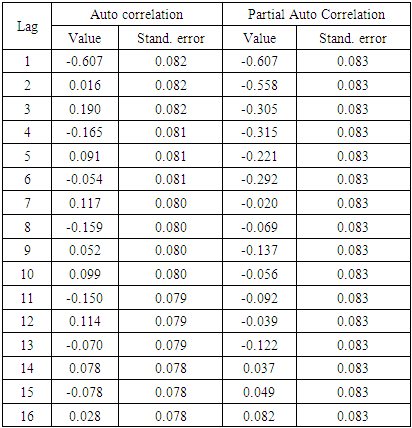
The values or the numbers of p and q of the model were identified depending on the autocorrelation and partial autocorrelation coefficients (ACF and PACFs) of various orders of Yt. p and q values were calculated and presented in Table 2 and Figure 3.Table 2. Auto Correlation Function and Partial Auto Correlation Function of Eggs Production of the Farm under Study
 |
| |
|
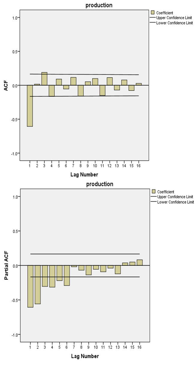 | Figure 3. AFC and PACF of differenced and logged eggs production data |
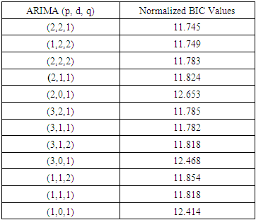
In the PACF chart, the number of lags exceeds 0.5 (positive or negative) was 2, and this suggested that (p order can be 2). In the ACF chart, the number of lags above 0.5 was 1, and this suggested that (q order equal 1) with difference equals 2.There were many ARIMA models which were suggested to represent the data with the normalized BIC values as in Table 3. The most fitted model was with the smallest normalized BIC value (11.745). Then the most suitable ARIMA model was with the order (2,2,1). Also, ARIMA model with ordering (1,2,2) is good in prediction process with BIC value (11.749) followed by (3,1,1), (2,2,2) and (3,2,1) of BIC values (11.782), (11.783) and (11.785) respectively.Table 3. Different ARIMA Models and the Corresponding Normalized BIC Values
 |
| |
|
3.2. Estimation of the Model Parameters
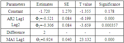
The parameters of (2, 2, 1) ARIMA model were presented in Table 4. In this model, the P value of the constant was > 0.05 (0.178) and this indicated that the model fitted without the constant. The other coefficients of AR and MA were also in Table 4. The values of the coefficients and the standard errors of AR and MA parameters were (-0.521 with 0.084 SE, - 0.306 with 0.084 SE and 0.924 with 0.040 SE) respectively. Their t values were (-6.199, -3.659 and 23.132). They were significantly differ from zero as their P values were (0.000, 0.000357 and 0.000) for AR at lag 1 and lag 2 and MA respectively. Then, this egg production model will be as follows: | (12) |
Where Yt is the predicted amount of egg at time t. Yt−1 is the predicted amount of egg of one previous day.Yt−2 is the predicted amount of egg of two previous day.εt−1 is the previous one day residual.Table 4. Parameters of the ARIMA Model (2,2,1) Fitted for Eggs Production
 |
| |
|
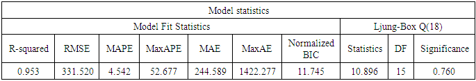
The other model statistics which indicated fitting of the model to the data were presented in Table 5. Higher R2 value (0.953) and higher MAPE value (4.542) with the lowest normalized BIC (11.745) and lower RMSE value (331.520). All these measures were a good indicator of fitting of the model to the data well.Table 5. Estimated ARIMA Model Fit Statistics
 |
| |
|
3.3. Diagnostic Checking of the Model
For checking the model adequacy the ACF and PACF of the residuals were graphed. The graphs of these residuals showed no specific information of the data appeared where all the points were irregularly distributed around zero (no systematic pattern) indicated that the model fitted was adequate as in Figure 4.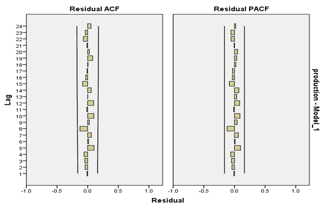 | Figure 4. Residuals of ACF and PACF |
The Ljung – Box (Q) statistic for testing of the residual of the model [14]. This statistic with a value of 10.896 for 15 d.f and its P-value equal 0.760 (the model was not significantly different from zero) as in Table 5. Then, the null hypothesis of white noise was accepted, and this meant that the model fitted is adequate as it absorbed all information of the data.
3.4. Using the Model in Forecasting Process
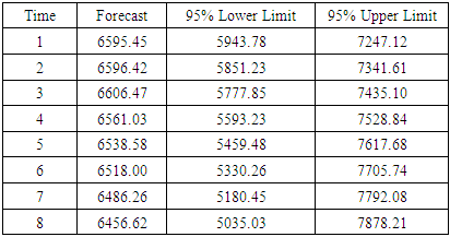
The actual and predicted values of egg production were shown in Table 6 and Figure 5. Forecasting process with the model (2,2,1) for forecasting i.e 8 days of future egg production indicated a good fitting of the model for prediction.Table 6. Statistics for Prediction of Egg Production
 |
| |
|
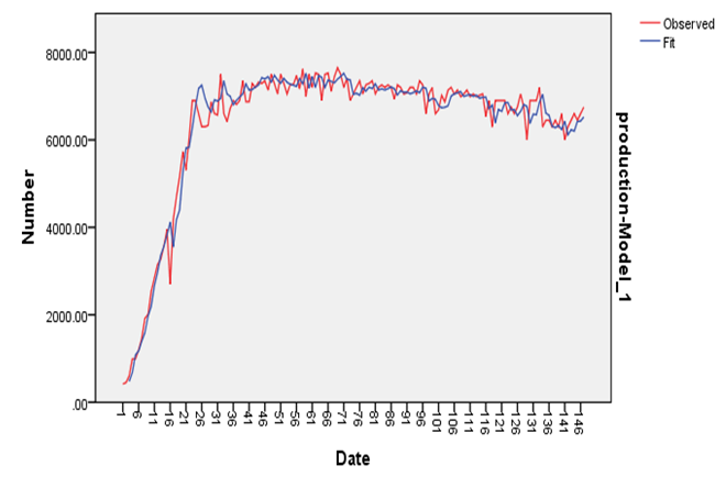 | Figure 5. Actual and estimated eggs production |
4. Conclusions
In this study the model of the best choice was ARIMA model with the order (2, 2, 1) as its R squared value was 0.95 (high value) and it had the lowest BIC values between the other models. It was noticed that egg production would increase as this model give evidence about future egg production. This model give information which are important in decision making process related to the future egg production in this farm. ARIMA model is a good model in forecasting the future performance not only for this farm but for egg producers all over the world.
References
| [1] | Makridakis, S., 1996, Forecasting: its role and value for planning and strategy, International Journal of Forecasting, 12(4), 513-537. |
| [2] | Eccles, M., Grimshaw, J., Campbell, M., Ramsay, C., 2003, Research designs for studies evaluating the effectiveness of change and improvement strategies, Quality Safety Health Care, 12, 47-52. |
| [3] | G.E.P. Box and J.M. Jenkins, Time Series Analysis - Forecasting and Control, San Francisco: Holden-Day Inc., 1970. |
| [4] | J. Shiskin, A.H. Young, and J.C. Musgrave, The X11 Variant of the Census Method II: Seasonal Adjustment Program, Technical Paper 15, US Department of Commerce, Bureau of the Census, 1967. |
| [5] | J. Jarrett, Business Forecasting Methods, 2nd edition, Basil: Blackwell. 1990. |
| [6] | M.O. Thomas, Short Term Forecasting, an Introduction to the Box Jenkins Approach, John Wiley & Sons, 1983. |
| [7] | P. Alan, Forecasting with Univariate Box–Jenkins Models - Concepts and Cases. New York: John Wiley, 1983, p. 81. |
| [8] | Chaudhari, D.J., Tingre, A. S., 2015, Forecasting eggs production in India, Indian J. Anim. Res., 49 (3), 367-372. |
| [9] | H. Akaike, On Entropy Maximization Principle in: Krishnaiah, P. R. (Editor), Application of Statistics, Amsterdam: North-Holland, 1977, p. 27-41. |
| [10] | Schwarz, G. E., 1978, Estimating the dimension of a model, Annals of Statistics, 6(2), 461-464. |
| [11] | R.S. Tsay, Analysis of Financial Time Series: Financial Econometrics. John Wiley & Sons, Inc., 2002. |
| [12] | Elivli, S., Uzgoren, N., Savas, M., 2009, Control charts for autocorrelated colemanite data, J.Sci. Indust Res., 68, 11-17. |
| [13] | Amin, M., Amanullah, M., Akbar, A., 2014, Time series modeling for forecasting wheat production of Pakistan, The Journal of Animal & Plant Sciences, 24(5), 1444-1451. |
| [14] | Ljung, G, Box, G. E. P., 1978, On a Measure of lack of fit in Time Series Models, Biometrika, 65, 553-564. |

 Abstract
 Reference
 Full-Text PDF
 Full-text HTML