Mohamed S. EL-Sherbeny1, 2, Zienab M. Hussien1
1Department of Mathematics, Faculty of Science & Arts, Rabigh- King AbdullAziz University, Rabigh, Saudi Arabia
2Department of Mathematics, Faculty of Science, Helwan University, Cairo, Egypt
Correspondence to: Mohamed S. EL-Sherbeny, Department of Mathematics, Faculty of Science & Arts, Rabigh- King AbdullAziz University, Rabigh, Saudi Arabia.
| Email: |  |
Copyright © 2018 The Author(s). Published by Scientific & Academic Publishing.
This work is licensed under the Creative Commons Attribution International License (CC BY).
http://creativecommons.org/licenses/by/4.0/

Abstract
This paper presents the reliability analysis of a two-compressor (non-identical) parallel system, which is part of the refrigeration system serving an ammonia storage tank. The failure rate of any compressor is a constant and the repair time distribution is a two-stage Erlanglan distribution. Measures of system performance such as reliability, system availability, and steady-state availability are derived. Also, a consistent asymptotically normal estimator and an asymptotic confidence interval for the steady-state availability and the mean time to failure of this system are obtained. Finally, a numerical example illustrates the results.
Keywords:
Mean time to system failure, Steady-state availability, Erlang distribution
Cite this paper: Mohamed S. EL-Sherbeny, Zienab M. Hussien, Interval Estimation of the Availability of a Two-Compressor with Erlangian Repair Time, Applied Mathematics, Vol. 8 No. 3, 2018, pp. 46-61. doi: 10.5923/j.am.20180803.03.
1. Introduction
Recent technological developments have given rise to the design of many complex systems containing several subsystems to perform different operations in various fields such as defence, industry and engineering systems. Because of the varied nature, these problems have attracted the attention of systems engineers and applied probabilists.Repairable systems were studied in the past with reference to the evaluation of their performance in terms of reliability and availability. Work (Claasen, S.J., Joubert & Yadavalli) [2] have considered a two-unit standby system with non-instantaneous switch-over and "dead time" and obtain exact confidence limits for the steady-state availability of system. In the work (Chandrasekhar, Natarajan & Yadavalli) [1] studied the two unit standby system and obtain exact confidence limits for the steady-state availability of system, when the failure rate of an operative unit is constant and the repair time of the failed unit follows a two stage Erlang distribution. The stochastic analysis of a non-identical two-unit parallel system with common-cause failure by graphical evaluation and review technique (GERT) considered by (Sridharan & Kalyani) [6]. The cost-benefit analysis of a two-unit cold standby system with two types of repair- minor (regular) and major (expert) are considered by [5, 9] studied the optimal system for series systems with mixed standby components. In the work (Wang, Liu & Pearn) [4] studied the availability analysis of three different series system configurations with warm standby components and general repair times. Work (Wang & Kuo) [3] has considered the reliability and availability characteristics of four different series system configurations with mixed standby.The purpose of the present paper is to study reliability analysis of a two-compressor arranging in parallel and find an estimator and asymptotic confidence interval for steady-state availability and mean time to failure of the system.
2. Description of the System
For the sake of discussion, we consider the system consists of two-compressor (A, B) (Fig.1) being part of the refrigeration system of an ammonia storage facility. Its function is to condense ammonia vapors coming from the tank, to maintain tank pressure at normal level, which is close to atmospheric pressure. After compression, condensation and expansion liquid cryogenic ammonia returns to the tank. We assume that two-compressor (non-identical) are arranged in parallel. In the beginning, the failure rate of a compressor A (B) is a constant with parameter  If compressor A (B) failed, the failure rate of B (A) is a constant with parameter
  The repair time distribution of two-compressor (A, B) is a two-stage Erlang distribution with parameter
  . Respectively, there is only one repair facility where the service discipline is FCFS. Whenever one of these compressors is operating online only and the other fails, the failed compressor goes to the repair. In the first stage, the repairing process of the compressor is started but it doesn’t complete, while the repairing process is completed in the second stage. Each compressor is assumed to be as new after repairment.
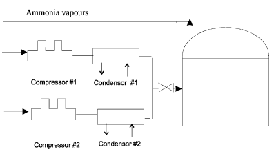 | Figure 1. Two-compressor system of a refrigeration system |
Since an Erlang distribution can be considered as the distribution of the sum of two independent and identically distributed exponential random variables, the stochastic process describing the behavior of the system is a Markov Process. Let 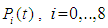 be the probability that the system is in state
  at time
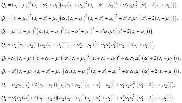
  . The infinitesimal generator of the Markov Process is given below.
 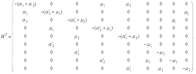 | (1) |
We assume that initially both the compressors are operable and obtain the measures of system performance.
3. System Availability
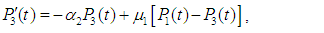
The system availability is the probability that the system operates within the tolerances at a given instant of time and is obtained as follows. Include the diagram for the infinitesimal generator for the system of ODEs for probabilities  ; eq. (1) and eqs. (2) to (10).
 | (2) |
 | (3) |
 | (4) |
 | (5) |
 | (6) |
 | (7) |
 | (8) |
 | (9) |
 | (10) |
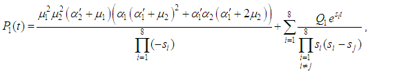
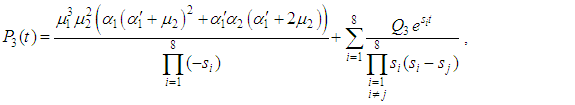
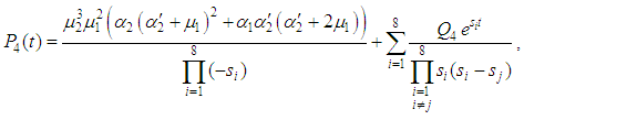
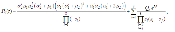
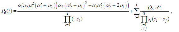
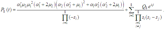
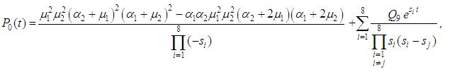
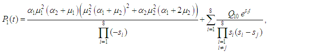
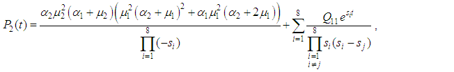
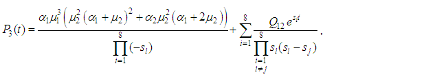
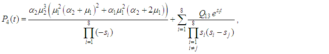
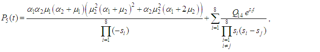
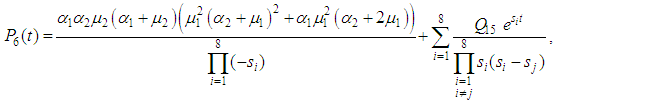
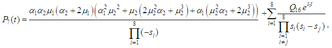
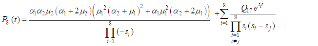
At time 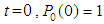 and all the other initial condition probabilities are equal to zero.Taking Laplace transforms on both the sides of the differential equations given above, solving for Laplace transforms and inverting, we get
 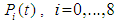 .
.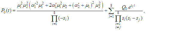 | (11) |
 | (12) |
 | (13) |
 | (14) |
 | (15) |
 | (16) |
 | (17) |
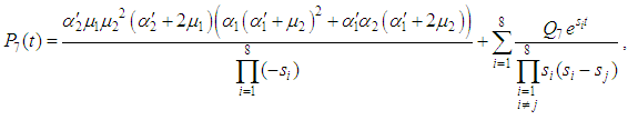 | (18) |
 | (19) |
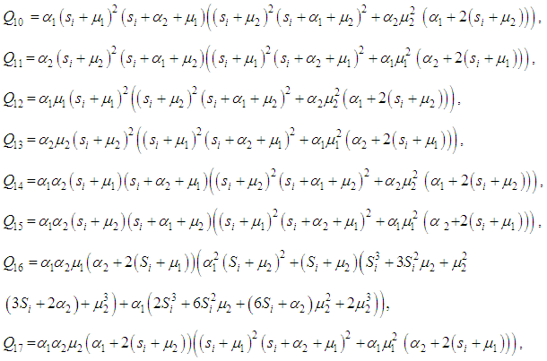
Where
 and
and  are the roots of the following equation:
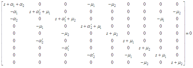 Since
Since  and
and  correspond to system up-states, the system availability is given by
 | (20) |
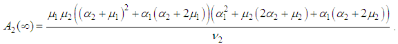
3.1. The Steady-state Availability
The steady-state availability of the system is given by  | (21) |
 | (22) |
where
 and,
and,

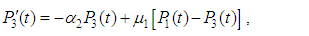
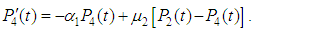
4. Reliability
The following differential equations associated with the system up states are obtained: | (23) |
 | (24) |
 | (25) |
 | (26) |
 | (27) |
At time  and all the other initial condition probabilities are equal to zero. By solving the above equations using Laplace transforms and inverting, we get
  . Then the system reliability is given by:
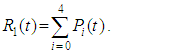 | (28) |
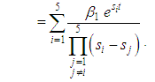 | (29) |
where, and
and  are the roots of the following equation:
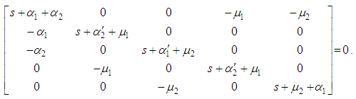 | (30) |
Now, we calculate the mean time to failure of the system by using the relation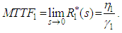 | (31) |
where,  and
and The variance of time to failure of the system is given by
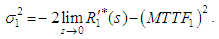 | (32) |
 is the derivative of
  with respect to s.
 | (33) |
where,
5. Special Case Model
When two units are independent (i.e.  ).
).
5.1. Availability of the System
We have | (34) |
 | (35) |
 | (36) |
 | (37) |
 | (38) |
 | (39) |
 | (40) |
 | (41) |
 | (42) |
At time  and all the other initial condition probabilities are equal to zero.Taking Laplace transforms on both the sides of the differential equations given above, solving for Laplace transforms and inverting, we get
 | (43) |
 | (44) |
 | (45) |
 | (46) |
 | (47) |
 | (48) |
 | (49) |
 | (50) |
 | (51) |
where,
 ,and
,and  are the roots of the following equation:
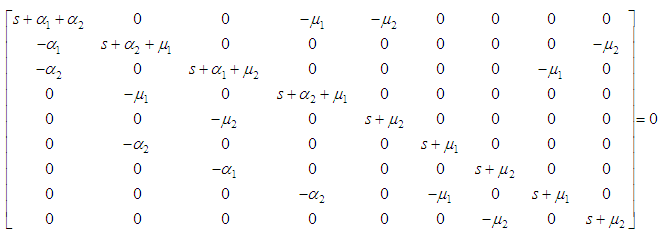 Since
Since  and
and  correspond to system up-states, the system availability is given by
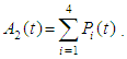 | (52) |
5.1.1. The Steady-state Availability
The steady-state availability of the system is given by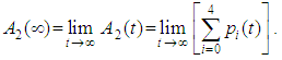 | (53) |
 | (54) |
where,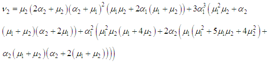
5.2. Reliability Analysis
The following differential equations associated with the system up states are obtained: | (55) |
 | (56) |
 | (57) |
 | (58) |
 | (59) |
At time  and all the other initial condition probabilities are equal to zero. By solving the above equations using Laplace transforms and inverting, we get
 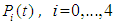 . Then the system reliability is given by:
 | (60) |
where,
 , and
, and  are the roots of the following equation:
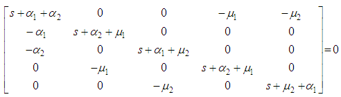 | (61) |
Now, we calculate the mean time to failure of the system by using the relation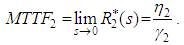 | (62) |
where, , and
, and The variance of time to failure of the system is given by
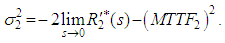 | (63) |
where  is the derivative of
  with respect to s.
 | (64) |
where 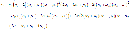 In the following sections, we obtain CAN estimator, a
  asymptotic confidence interval for the steady state availability of the system and an estimator of the system reliability.
6. Confidence Interval for Steady-State Availability of the System
Let  be random samples of size
  each drawn from different exponential populations with first (A) compressor’s failure rate
  second (B) compressor’s failure rate
  The failure of compressor B changes the parameter of exponential lifetime of A from
  to
to  , while the failure of component A changes the parameter of exponential lifetime of B from
  to
to  If
If  is the parameter of the exponential distribution, then an estimate can be found for either
  or for the parameter
 , which is equal to the mean value of the time of failure. For the analysis, let
  The maximum likelihood estimator (MLE) of
  is given by
  Similarly
  and
and  are the MLE’s of
  and
and  respectively.Moreover, Let
  be random samples of size
  each drawn from different Erlang populations with first unit’s repair rate
  and second unit’s repair rate
  If µ1 is the parameter of the Erlangian distribution, then an estimate can be found for either µ1, or for the parameter
  , which is equal to the mean value of the time of the failure time. For the analysis, let
  .The maximum likelihood estimator (MLE) of
  is given by
  Similarly
  is the MLE’s of
  .Hence, the MLE of
  | (65) |
where

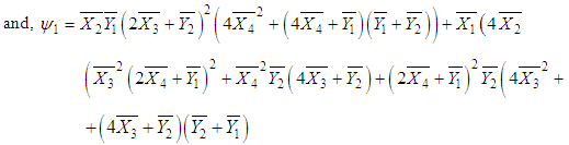 It should be noted that
  is real valued differential function in
  and
and  Now consider the following application of the multiplicative central limit theorem (Rao, 1973), it follows that
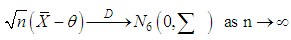 where
where and the dispersion matrix
  is given by
 According to center limit theorem, see (Rao, 1973), as
  ,we have
 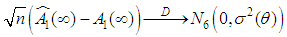 where
where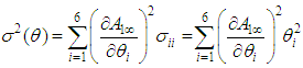 Consequently
  is estimator of
  :Let
:Let  be the estimator of
  obtained by replacing
  by a consistent estimator
  namely.
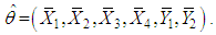 By Slutskey’s theorem
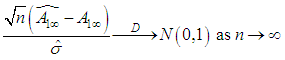 That is,
 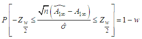 Where
Where  is obtained from normal tables. Hence, a
  asymptotic confidence interval for
  is given by
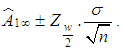
7. Confidence Limits Interval for Mean Time to Failure of the Systems
Since, the maximum likelihood estimator (MLE) of  is given by
  Similarly
  and
and  are the MLE’s of
  and
and  respectively. Also, the maximum likelihood estimator (MLE) of
  is given by
  similarly
  are the MLE’s of
  .Hence, the MLE of
  | (66) |
where and,
and, It should be noted that
  is real valued differential function in
  and
and  Now consider the following application of the multiplicative central limit theorem (Rao, 1973), it follows that
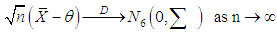 where
where and the dispersion matrix
 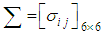 is given by
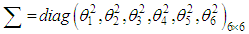 According to center limit theorem, see (Rao, 1973), as
  ,we have
 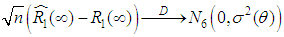 where
where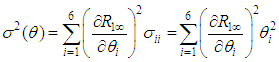 Consequently
  is estimator of
  Let
Let  be the estimator of
  obtained by replacing
  by a consistent estimator
  namely.
 By Slutskey’s theorem
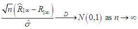 That is,
 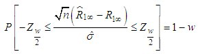 Where
Where  is obtained from normal tables. Hence, a
  asymptotic confidence interval for
  is given by
 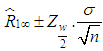 .
.
8. Confidence Interval for Steady-State Availability of the Special Case Model
Let 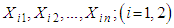 be random samples of size
  each drawn from different exponential populations with first unit’s failure rate
  and second unit’s failure rate
  . If α1 is the parameter of the exponential distribution, then an estimate can be found for either α1, or for the parameter
  , which is equal to the mean value of the time of the failure time. For the analysis, let
  .The maximum likelihood estimator (MLE) of
  is given by
  Similarly
  is the MLE’s of
  .Moreover, Let
  be random samples of size
  each drawn from different Erlang populations with first unit’s repair rate
  and second unit’s repair rate
  . If µ1 is the parameter of the Erlangian distribution, then an estimate can be found for either µ1, or for the parameter
  , which is equal to the mean value of the time of the failure time. For the analysis, let
  The maximum likelihood estimator (MLE) of
  is given by
  Similarly
  is the MLE’s of
  .Hence, the MLE of
  | (67) |
where and,
and,  It should be noted that
  is real valued differential function in
  and
and  Now consider the following application of the multiplicative central limit theorem (Rao, 1973), it follows that
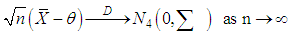 where
where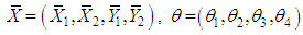 and the dispersion matrix
 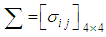 is given by
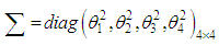 According to center limit theorem, see (Rao, 1973), as
  ,we have
 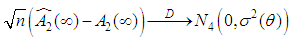 where
where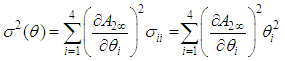 Consequently
  is estimator of
  :Let
:Let  be the estimator of
  obtained by replacing
  by a consistent estimator
  namely.
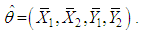 By Slutskey’s theorem
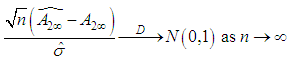 That is,
 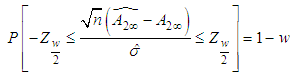 Where
Where  is obtained from normal tables. Hence, a
  asymptotic confidence interval for
  is given by
9. Confidence Limits Interval for Mean Time to Failure of the Special Case Model
Since, the maximum likelihood estimator (MLE) of  is given by
  similarly
  are the MLE’s of
  . also, the maximum likelihood estimator (MLE) of
  is given by
  similarly
  are the MLE’s of
  .Hence, the MLE of
  | (68) |
where and,
and, It should be noted that
  is real valued differential function in
  and
and  Now consider the following application of the multiplicative central limit theorem (Rao, 1973), it follows that
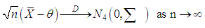 where
where and the dispersion matrix
  is given by
 According to center limit theorem, see (Rao, 1973), as
  ,we have
 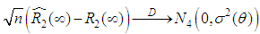 where
where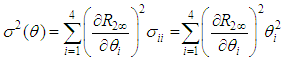 Consequently
  is estimator of
  :Let
:Let  be the estimator of
  obtained by replacing
  by a consistent estimator
  namely.
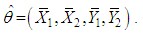 By Slutskey’s theorem
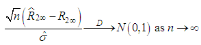 That is,
 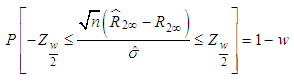 Where
Where  is obtained from normal tables. Hence, a
  asymptotic confidence interval for
  is given by
  .
.
10. Study of System Behavior through Graphs
We plot the MTTF and steady-state availability for the two models (system model and special case model), against  and
and  . These curves are shown in Figures 2 –3.
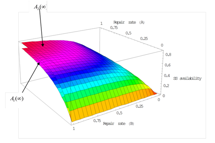 | Figure 2. S.S. Availability vs. Repair rate(A)  Repair rate(B) Repair rate(B)  |
From Figure (2) we conclude that, as the repair time rate  is increase and the repair time rate
  is increase, the steady-state availability is increases. When the steady-state availability of special case
  is greater than the system steady-state availability
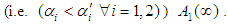
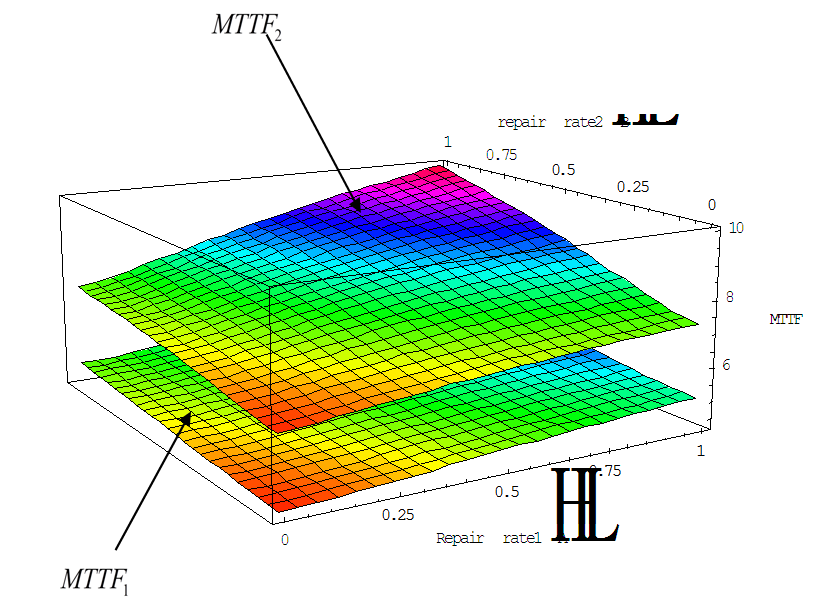 | Figure 3. MTTF vs. Repair rate(A)  Repair rate(B) Repair rate(B)  |
In Figure (3) it is seen that, as the repair time rate  is increase and the repair time rate
  is increase, the mean time to failure of the system
  is increases. The mean time to failure of special case (i.e.
  )
)  is better than The mean time to failure of the system
  Therefore, for achieving high reliability of the system, we recommend that the two-compressor are independent (i.e. the failure rate of compressor is constant
 ), this is clear in the graphs.
References
| [1] | Chandrasekhar, P., Natarajan, R., and Yadavalli, V. S. S., (A Study on a two unit standby system with Erlangian repair time). Asia-Pacific Journal of Operational Research, Vol. 21, No. 3, pp. 271-277, 2004. |
| [2] | Claasen, S.J. Joubert, J.W. and Yadavalli, V.S.S., (Interval estimation of the availability of a two-unit standby system with non-instantaneous switch-over and Dead time). Pak J. Statist., Vol. 20(1) pp 115 – 122, 2004. |
| [3] | Kuo-Hsiung Wang, Ching-Chang Kuo., (Cost and probabilistic analysis of series systems with mixed standby components). Applied Mathematical Modelling 24: 957 –967 , 2000. |
| [4] | Kuo-Hsiung Wang, Yi-Chun Liu, Wen Lea Pearn., (Cost benefit analysis of series systems with warm standby components and general repair time). Math Meth Oper Res 61:329–343, 2005. |
| [5] | M. Rashad, M. Salah El-Sherbeny, and Z. M. Hussien., Cost Analysis of a Two-unit Cold Standby System With Imperfect Switch, Patience Time and Two Type of repair, J. Egypt Math. Soc. 17 (1) (2009) 65-81. |
| [6] | M. Salah El-Sherbeny., The optimal system for series systems with mixed standby components, Journal of Quality in Maintenance Engineering, 16 (3) (2010). |
| [7] | Sridharan,V., Kalyani,T. V, (Stochastic analysis of a non-identical two- unit parallel system with common-cause failure using GERT technique). Information and Management Sciences., Vol. 13, No. 1, pp. 49-57, 2002. |

 Abstract
 Reference
 Full-Text PDF
 Full-text HTML