Pakhshan Mohammed Ameen Hasan, Nejmaddin Abdulla Suleiman
Department of Mathematics, College of Education, Salahaddin University- Hawler, Kurdistan Region, Iraq
Correspondence to: Pakhshan Mohammed Ameen Hasan, Department of Mathematics, College of Education, Salahaddin University- Hawler, Kurdistan Region, Iraq.
| Email: |  |
Copyright © 2018 The Author(s). Published by Scientific & Academic Publishing.
This work is licensed under the Creative Commons Attribution International License (CC BY).
http://creativecommons.org/licenses/by/4.0/

Abstract
In this paper, a new technique is presented for solving linear mixed Volterra-Fredholm integral equations of the second kind. This technique is based on a polynomial of degree n and on the conversion of the integral equation to a linear programming problem, which will be solved by the Simplex method. For more illustration, an algorithm is suggested, and applied on several examples. The program is written in MATLAB (R2015a) to compute the results. To show the competency of the method and the accuracy of the results, comparison between the exact and the approximate solution are given by computing the absolute error and the least square error (L.S.E.).
Keywords:
Linear programming problem (LPP), Mixed linear Volterra-Fredholm integral equation of the second kind (MLV-FIE2nd), Simplex method
Cite this paper: Pakhshan Mohammed Ameen Hasan, Nejmaddin Abdulla Suleiman, Numerical Solution of Mixed Volterra-Fredholm Integral Equations Using Linear Programming Problem, Applied Mathematics, Vol. 8 No. 3, 2018, pp. 42-45. doi: 10.5923/j.am.20180803.02.
1. Introduction
Integral equations are found in different fields of science and several applications in approximation theory, fluid dynamics, electrodynamics, medicine, etc.Recently, several works have been devoted to the existence of the solution of mixed type of Volterra-Fredholm integral equations [1, 3, 8]. The analytical solution of this type of integral equation is obtained in [1, 9, 11], while the numerical methods takes an important place in solving them [5, 7, 10, 14, 16, 17].The linear mixed Volterra-Fredholm integral equation of the second kind (LMV-FIESK), which has the form | (1) |
is considered in this paper, where the free term f and the kernel k are known, while u(x) is the unknown function which will be found.In [3], Ibrahim, et al. used new iterative method for solving the mixed Volterra-Fredholm integral equations. Wang treated this problem in [6] by using Taylor collocation method. In [12], Shahooth solved the Volterra-Fredholm integral equations of the second kind by using Bernstein polynomials method. In addition, Ezzati and Najafalizadeh, used Cas wavelets for solving Volterra-Fredholm integral equations in [14]. Throughout this work, the central problem is the approximation of  by a function whose general form
  depends on n parameters
  . By choosing approximate values
 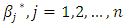 of these parameters according to some appropriate approximation criterion, we obtain a particular approximating function
  of the equation (1).
2. Fundamental Concepts [2, 11]
2.1. Linear Programming Problem (LPP)
It is one of the most important optimization (maximization\ minimization) techniques developed in the field of operations research. More formally, linear programming is a technique for the optimization of a linear objective function (obj.fn.) subject to linear equality and\or inequality constraints, where the variables are nonnegative. In general, a linear programming model is defined as follows: subject to
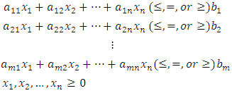 The required smallest (or largest) value of the objective function is called the optimal value and the variables
  that give the optimal solution are called the decision variables.
3. The Method
An important class of methods for solving integral equations involve substitution of a suitable approximation function  in place of the unknown solution
  . Here the key to effective approximating lies in the selection of the appropriate general form of
  in the form
 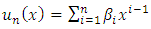 | (2) |
The values of  are then determined using the transformation
  which arises from substituting this function in the integral equation (1), which yields
  | (3) |
Thus | (4) |
Let 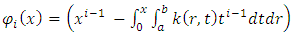 | (5) |
Thus equation (4) becomes: 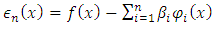 | (6) |
One way of improving this technique is to select  points
  and solve the over determined system of linear equations
 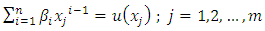 | (7) |
This allows us to represent the function u(x) on more than (n) points of [a, b], when determining  Further, for problem (7) a solution always exists in the following sense.Let the residuals of equation (7) be defined as
 | (8) |
and 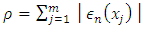 | (9) |
Consider the problem of determining 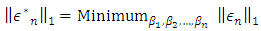 | (10) |
where 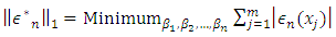 | (12) |
By substituting equation (8) in equation (12), we get | (13) |
The quantity  always exists and the optimal values of
  yield a best
  (least-first-power) solution to equation (1). Thus a general technique for determining
  solution to the LMV-FIESK is available which is based on solving the equivalent problem
  subject to
 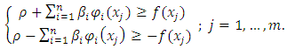 | (14) |
 are unrestricted in sign. The approximate values
  of
of  which are calculated in (14) give an approximate solution of equation (1) as
 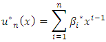 In practice we do not solve (14) exactly, but alternatively a corresponding discrete problem is solved using the Simplex method of Linear Programming.
4. The Algorithm
To find an approximate solution of (LMV-FIESK) perform the following steps: Step 1: select two positive integers n and m.Step 2: compute  Step 3: calculate
  in equation (5) for all
  and
and  Step 4: use equation (9) to compute
  , and then construct the objective function
  of the LPP.Step 5: construct the constraints of the LPP from equation (14).Step 6: use the Simplex method to find optimal approximate values
  of
of  Step 7: substitute these values of
  in the equation (2) to determine the approximate solution of equation (1).
5. Numerical Examples
In this section, several examples will be solved to show the accuracy of our approach.Example 1. Consider the (MLV-FIE2nd)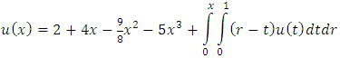 whose exact solution is
 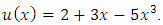 Applying the algorithm of the described method with n=4 and 2m=8 constraints will convert the integral equation to the following LPP:
 subject to
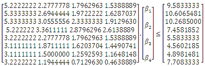 where
where  are unrestricted in sign, which will be solved by the Simplex method to get the values of
  Thus
Thus  Putting these values in equation (2) produces the approximate solution
  In this case the least square error (L.S.E.) is
  Increasing the value of m and taking m=6>n, will give a LPP with 4 unknowns and 12 constraints. Use the Simplex method to get the values of
  then put them in equation (2) to get the approximate solution
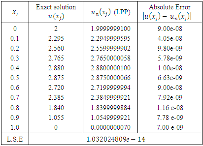
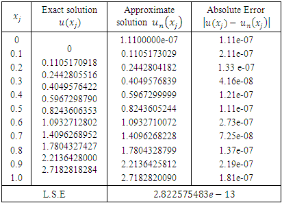
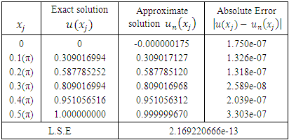
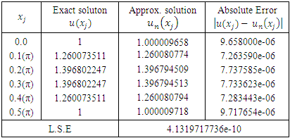
 In Table (1), the real solution and the corresponding approximate solution using (LPP) are obtained; also the values of the absolute error and (L.S.E) are presented.
Table 1. The LPP results compared with exact solutions for n=4 and m=6
 |
| |
|
Example 2. The integral equation 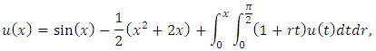 has the exact solution
  Assume that the approximate solution is of the form
 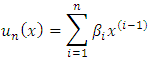 By following the steps of the algorithm and choosing different values of n and m, we will get the results of L.S.E. that are listed in Table (2).
 Table 2. The L.S.E. of Example 2 for different values of n and m
 |
| |
|
while, taking n=8 and m=10, gives the approximate solution 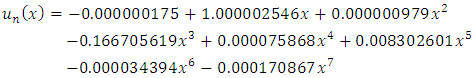 Table (3) presents the comparison between the exact and the numerical solutions with n=8, and m=10.
Table 3. The comparison between the exact and the numerical solutions
 |
| |
|
Example 3. Consider the MV-FIE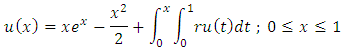 the exact solution is
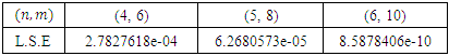
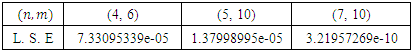
  Performing the prescribed steps in the algorithm with different values of (n, m), we get the results that are listed in Table (4).
Table 4. L.S.E. of Example (3) with different values of n and m
 |
| |
|
while, taking n=8 and m=10, gives the numerical solution 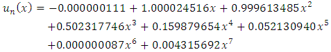 Table (5) presents the comparison between the exact and the numerical solutions for n=8, and m=10.
Table 5. The comparison between the exact and the numerical solutions
 |
| |
|
Example 4. Consider the MV-FIE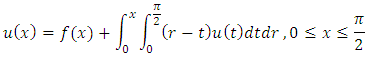 Where
Where 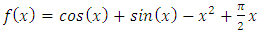 and the exact solution
 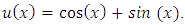 Applying the algorithm of the LPP with n=6 and m=9 we get a LPP with 6 unknowns and 18 constraints which can be solved by the Simplex method, and then we get the results that shown in Table (6).
 Table 6. The comparison between the exact and the numerical solutions
 |
| |
|
6. Conclusions
In this paper, the linear programming method is introduced to solve the second kind mixed Volterra–Fredholm integral equations. Several examples are applied for illustration and good approximate results are found. Moreover, the results of (LPP) are compared with the exact solutions to demonstrate the implementation of the method. Also, it is claimed that better results can be obtained by increasing both the number of basis functions (n) and the number of constraints (m>n). The given numerical examples and the outcomes in Tables (1-6) support these claims.
References
| [1] | A. Aghajani, Y. Jalilian, Existence and global attractivity of Solution of a nonlinear functional Integral Equations, Communications in Nonlinear science and Numerical Simulation 15 (2010), 3306-3312. |
| [2] | H. Taha, Operations Research, United States of America. (1976), pp. 28-32. |
| [3] | H. Tidke, Iexistence and Uniqueness of Continuous Solution of Mixed Type Integral Equations in Cone Metric Space, Kathmandu University Journal of Science, Engineering and Technology,7(1), 48-55, (2011). |
| [4] | H. Ibrahim, F. Attah, and G.T. Gyegwe, On the solution of Volterra-Fredholm and mixed Volterra-Fredholm integral equations using the new iterative method. Applied Mathematics, 6 (1): 1-5 (2016). |
| [5] | K. Maleknejad, M. Hadizadeh, A New Computational Method for Volterra-Fredholm Integral Equation, J. Comput. Math. Appl. 37 (1999), 37-48. |
| [6] | K. Wang, Q. Wang, Taylor Ollocation Method and Convergnce Analysis for the Volterra-Fredholm Integral Equations, Journal of Computational and Applied Mathematics, 260 (2014) 294-300. |
| [7] | L.M. Delves, J. Walsh, Numerical Solution of Integral Equations. Oxford. (1974), pp. 97-106. |
| [8] | M.A. Abdou, G.M. Abd Al-Kader, Mixed Type of Fredholm- Volterra Integral Equation, Le Matematiche, LX (2005), pp. 41-58. |
| [9] | M.A. Abdou, Integral Equation of Mixed Type and Integrals of Orthogonal Polynomials, J.Comp. Appl. Math. 138 (2002), 273-285. |
| [10] | M.A. Abdou, K.I. Mohamed, A.S. Ismail, On the Numerical Solution of Fredholm-VolterraIntegral Equation, Appl. Math. Comput. 146 (2003) 713-728. |
| [11] | M.A. Abdou, On Asymptotic Method for Fredholm-Volterra Integral Equation of the Second Kind in Contact problem, J. Com. Appl. Math. 154 (2003), 431-446. |
| [12] | M. Shahooth, Numerical Solution for Mixed Volterra-Fredhlm Integral Equations of the Second Kind By Bernstein Polyno- mials Method, Mathematical Theory and Modeling, 5 (10) 154-162 (2015). |
| [13] | Q. Wang, K. Wang, and S. Chen, Least Square Approximation Method for the Solution of Volterra-Fredholm Integral Equations, Journal of Computational and Applied Mathematics, 272 (2014), 141-147. |
| [14] | R. Ezzati, S. Najafalizadeh, Numerical Methods for Solving Linear and Nonlinear Volterra-Fredholm Integral Equations by Using Cas Wavelets, World Applied Sciences Journal 18 (12): 1847-1854, (2012). |
| [15] | S. D. Sharma, Operations Research, Meerut, U.P. India. (1989), pp. 3-7. |
| [16] | S.S. Ahmed, Numerical Solution for Volterra-Fredholm Integral Equation of the Second Kind by Using Least squares technique, Iraqi Journal of Science, 52 (2011), pp.504-512. |
| [17] | Z. Chen, W. Jiang, An Approximate Solution for a Mixed Linear Volterra-Fredholm Integral Equations, Applied Mathematics Letter, 25 (2012) 1131-1134. |

 Abstract
 Reference
 Full-Text PDF
 Full-text HTML