I. M. Esuabana1, U. A. Abasiekwere2
1Department of Mathematics, University of Calabar, Calabar, Cross River State, Nigeria
2Department of Mathematics and Statistics, University of Uyo, Uyo, Akwa Ibom State, Nigeria
Correspondence to: I. M. Esuabana, Department of Mathematics, University of Calabar, Calabar, Cross River State, Nigeria.
| Email: |  |
Copyright © 2018 The Author(s). Published by Scientific & Academic Publishing.
This work is licensed under the Creative Commons Attribution International License (CC BY).
http://creativecommons.org/licenses/by/4.0/

Abstract
One of the most recent mathematical concepts, the regularization methods for solving integral equations, has brought in yet another dimension into the existing problems and has helped to usher in a new body of knowledge for further consideration. Indeed, new inputs have placed other numerical methods for solving integral equations in the fastest lane, since a number of methods were analysed with respect to accuracy, convergence and stability properties. Most of the work was done on the assumptions that the kernel  and the right-hand side
  are known without error and that the approximating equation can be exact, whereas, as is often the case, these may not be true. Consequently, the effect can be observed in the study of regularization methods for solving Volterra type integral equations of the first kind. Classical regularization methods tend to destroy the non-anticipatory (or causal) nature of the original Volterra problem because such methods typically rely on the computation of the Volterra adjoint operator. In this paper, we highlight the general concept of the regularization method of solution for Volterra integral equation of the first kind without destroying the Volterra structure.
Keywords:
Volterra Integral Equation, Regularization method, Ill-posed
Cite this paper: I. M. Esuabana, U. A. Abasiekwere, A Survey of Regularization Methods of Solution of Volterra Integral Equations of the First Kind, Applied Mathematics, Vol. 8 No. 3, 2018, pp. 33-41. doi: 10.5923/j.am.20180803.01.
1. Introduction
The theory of integral equations is interesting, not only in itself but also in the absolute importance of its results in the analysis of numerical methods of solution of various equations. Besides the concept of existence and uniqueness with respect to differential equations, the theory is concerned, in particular, with questions of regularity and stability of their solutions.In the last two and a half decades, there has been a tremendous increase in the applications of first kind integral equations of Volterra type. Among the areas where the applications of such class of equations abound in the natural sciences is the problem of restoration of incoming signals at the entrance of measuring instruments and observatory systems which, in view of their physical nature, allow some distortions of the observed and registered data [1].An integral equation is a functional equation in which the unknown function appears under one or several integral signs. In an integral equation of Volterra type for instance, the integrals containing the unknown function are characterized by a variable upper limit of integration. To be more precise, an integral equation of the form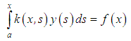 | (1) |
is called a linear Volterra integral equation of the first kind, or that of the form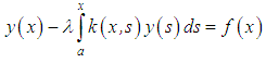 | (2) |
is called a linear Volterra integral equation of the second kind. Here,  are real numbers,
  is a parameter,
  is an unknown function, while
 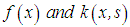 are given functions which are square integrable on
  and in the domain
  respectively. The function
  is called the free term, while the function
  is called the kernel.One distinguishing feature associated with this class of equations is the uncertainty surrounding their nature and this is reflected in the difficulties encountered when attempting to find their solutions using one or the other of the existing numerical methods [2]. On one hand, Volterra integral equations of the first kind appear to be special cases of Fredholm integral equations of the first kind and are consequently classified among the lists of ill-conditioned problems solvable by the classical regularization means. On the other hand, given a set of limitations (for example, given that their kernels and right-hand sides are “good” and “smooth”) Volterra integral equations of the first kind belong to the class of well-posed problems and hence can be solved through any direct method based on the discretization of the unknown solutions. Both approaches seem to be a little on the extreme. The use of discretization process transforms Volterra integral equations of the first kind into another problem (often systems of linear equations and may be solved by the well-known singular value decomposition) that can lead to solutions which may or may not deviate strongly from the (minimum norm) solution of the original equation [3]. A complete regularization (with its accompanying difficulties and unresolved questions) turns out to be a too complicated approach as it is observed that the methods for Volterra equations of the first kind are not nearly as ill-posed as methods for Fredholm integral equations of the first kind.In this study, we investigate the regularization methods with a view to identifying the properties and types that can be used in solving Volterra type equations of the first kind, but without destroying the Volterra structure. The methods in view are perhaps the discrete regularization methods. The discrete approximation methods provide another approach to regularize the original problem. In this case, the regularization parameter is the discretization parameter (or step size) and coordination between this parameter and the amount of noise
  in the problem is required to obtain good approximations in the presence of noise.
2. The Concept of a Regularizing Operator
We are already aware of the fact that the problem of solving Volterra integral equations of the first kind in some spaces, for example, in the triple (C,V,C) is, to a certain extent, ill-posed. Even in those spaces where the problems are well-conditioned, for example, in the space (C,V,C(1)), we still encounter significant difficulties, leading to some slight instabilities in the results during actualization. Consequently, to improve on the stability of the solutions which implies the accuracy of the desired results, we go out for the most stable methods. Among such methods are the regularization methods.Methods for construction of approximate solutions of ill-posed problems that are stable with respect to small perturbations of the initial data are referred to as regularization methods. The approach is based on what is called the fundamental concept of a regularizing operator [4]. In what follows, we examine the concept in detail.Suppose the operator A in the equation | (3) |
where Y and F are some metric spaces and A is a continuous operator mapping Y into F, is such that its inverse  is also continuous in the set
  and the set Y of possible solutions, is not compact.If the right–hand member of the equation is an element
  that differs from the exact right–hand member
  by no more than
  , that is, if
  , it is obvious that the approximate solutions
  of equation (3) cannot be defined as the exact solution of this equation with approximate right–hand member
  , that is, according to the formula
  .The numerical parameter
  characterizes the error in the right–hand member of equation (3). Therefore, it is natural to define
  with the aid of an operator depending on a parameter having a value chosen in accordance with the error
  in the initial data
  . Specifically, as
  , that is, as the right–hand member
  of equation (3) approaches (in the metric of the F) the exact value
  , the approximate solution
  must approach (in the metric of the space) the exact solution
  that we are seeking for in the equation
  .Now, assuming that the elements
  and
and  are connected by
  , we define the following concepts:Definition 2.1. An operator
  is said to be a regularizing operator for the equation
  in a neighbourhood of
  if:i) there exists a positive number
  such that the operator
  is defined for energy
  in
in  and every
  such that
  ii) for every
  , there exists a
  , such that the inequality
  implies the inequality
  , where
  Definition 2.2. An operator
  depending on a parameter α is called a regularizing operator for the equation Ay = f in a neighbourhood of
  if:i) there exists a positive number
  such that the operator
  is defined for every
  and every
  for which
  ii) there exists a function
  of
of  such that, for every
  , there exists a number
  such that the inclusion
  and the inequality
  imply
imply  where
where  Again, there is no assumption of the uniqueness of the operator
  . It is easy to point out here that the function
  also depends on
  .If
.If  , we know from studies by Tikhonov [4] that we can take for an approximate solution of equation (3) with approximately known right–hand member
  the element
  obtained with the aid of the regularizing operator
  where
where  in accordance with the error in the initial data
  . This solution is called a regularized solution of equation (3). The numerical parameter α is called the regularization parameter. Obviously, every regularizing operator defines a stable method of approximate construction of the solution of equations (3) provided the choice of α is consistent with the accuracy
  of the initial data
  . If we know that
  we can, by definition of a regularizing operator, choose the value of the regularization parameter
  in such a way that, as
  , the regularized solution
  approaches (in the metric of Y) the desired exact solution
  , that is,
  . This justifies taking as an approximate solution of equation (1) the regularized solution. Thus, the problem of finding an approximate solution of equation (1) that is stable under small changes in the right–hand member reduces to:i) finding regularizing operators;ii) determining the regularization parameter α from the supplementary information pertaining to the problem, for example, the size of the error in the right–hand member
  .This method of constructing approximate solutions is called the regularization method.Out of all the operators
  from F and Y that depend on the parameter α and which are defined for every f∈F and every positive α, we need to single out the operators that are continuous with respect to f. In doing this, we can give sufficient conditions for belonging to the set of regularizing operators of equation (3). This is an immediate consequence of the following theorem.Theorem 2.1. Let A denote an operator from Y into F and let
  denote an operator from F into Y that is defined for every element f∈F and every positive α that is continuous with respect to f. If
  for every element y∈Y, then the operator
  is a regularizing operator for the equation
  Proof. It will be sufficient to show that the operator
  possesses property (ii) of Definition 2.2.Let
  and
and  denote fixed elements of Y and F respectively such that
  . Let
. Let  denote a fixed positive number. Then, for every element
  such that
  , we have
 | (4) |
Since the operator  is continuous with respect to f at the “point”
  , it follows that, for sufficiently small positive
  , the inequality
 | (5) |
implies the inequality | (6) |
where  .Since
  it holds that
 | (7) |
 and
and  with
with  It follows from inequalities (4), (6), and (7) that, for every
  and
and  ,
, | (8) |
Since  there exist for every
  , a
, a  such that, for
  and
and  , inequalities (5) and (8) imply
  This completes the proof of Theorem 1.
3. Regularization Methods
3.1. Tikhonov’s Regularization Method
Consider the Volterra integral equation of the first kind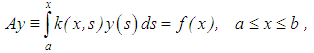 | (9) |
where To ensure the stability of the solution of equation (9), we introduce the condition of minimum smoothing functional given as
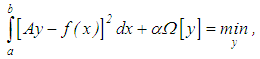 | (10) |
where, as it is so – called, the stabilizing functional, Ω[y], is usually written in the form [3]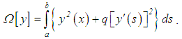 | (11) |
What is more, α > 0 is called the regularization parameter,  defines the order of the regularization (zero order if
  and first order if
  ). Expanding condition (10) using condition (11) and bearing in mind the Volterra structure of equation (9) yields the following equation of the second kind:
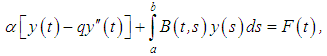 | (12) |
 where
where | (13) |
 | (14) |
and | (15) |
Expressions (13) and (14) may be written in another form as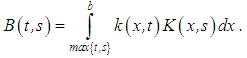 | (16) |
In place of equations (12) - (16), we may use the relation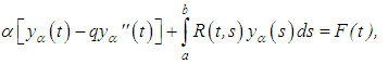 | (17) |
 where
where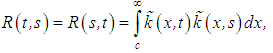 | (18) |
 | (19) |
and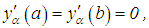 | (20) |
are valid for Fredholm first kind equation and setting in the later,  and
and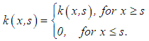 | (21) |
In all the cases considered above, the original Volterra integral equations of the first kind are replaced with equations of the second kind (precisely, integro-differential equation of the second kind) of Fredholm type. Consequently, the Tikhonov’s regularization method results in the loss of the Volterra structure but assists in the preliminary transformation of equation (10) (using, for example, the finite sum and the finite difference methods) into a system of linear algebraic equations with a full (positive definite) matrix (not triangular). This calls for a reasonable loss of time when solving it using any computational device. In spite of all these shortcomings, the use of Tikhonov’s regularization method in the solution of equation (9) still turns out to be one of the most effective of the regularization methods.
3.2. Tikhonov’s Regularization Method for Equation of Convolution type (Sequential Tikhonov Regularization Method)
We consider the convolution type Volterra integral equation of the first kind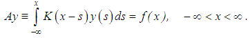 | (22) |
A complete discussion on this question has been provided by Savelova ([5], [6], [7], [8], [9], [10], [11]).For the convolution type Volterra integral equation of the first kind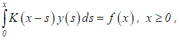 | (23) |
We first make use of the so-called techniques of extension [12]. We introduce the functions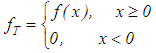 and
and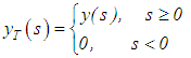 and hence obtain from equation (23), a new statement
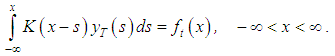 It is only from this moment that the Tikhonov’s regularization method may be applied.
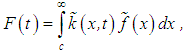
3.3. Denisov’s Regularization Method
Consider the equation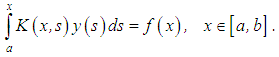 | (24) |
Let  and the functions
  be continuous and the exact solution
  . What is more, let it be given that
  Suppose further, that in place of the right member
  the approximate right member
  such that
  is known. Then, in place of equation (24), we propose the solution of the
  -regularizing equation
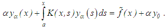 | (25) |
Such a procedure is close to the Lavrent-ev’s classical method. The asymptote of the solution of equation (25) is examined in the study by Blondel [13] when  with the exact function
  (but without the term
  ).In the study by Denisov [14], it is proved that
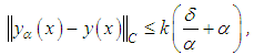 | (26) |
where k = constant. When  we select
  such that
  For instance, if
  is chosen so that
 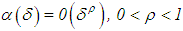 , we observe that
 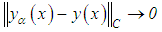 , which is the algorithm obtained from equation (24).We introduce yet another value of
  (call it the quasi-optimal regularizer and denote it by
  ), the minimizer of the right-hand side of equation (25). Hence, we obtain
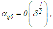 | (27) |
 | (28) |
An important feature of the method under consideration is the simple nature of equation (24). Furthermore, the Volterra structure of the original equation (as seen) is maintained. However, the method insists on an initial knowledge of the value of  which, in a concrete situation, is not obtainable.
3.4. Apartsin’s  Regularization Method
Further modification of Denisov’s  regularization method in conjunction with Apartsin–Bakushinskii’s
  regularization method is called
  regularization method. In the said
  regularization method, it is clear from the onset that the procedure will involve the replacement of the integral of equation (24) with the corresponding approximate finite sum ( h-regularization) on the grid and instead of battling with the identification of the preconceived appropriate values of
  and
and  , a system of linear algebraic equations is put in place of equation (24) and is independent of
  Now, we consider a system of linear algebraic equations with a triangular matrix of coefficients:
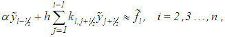 | (29) |
where Notice that the system in equation (28) is obtained by replacing the integral in equation (24) with a finite sum defined by the mid-point rectangular formula having a step-size of h = constant.Let
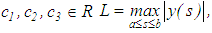
  and
and 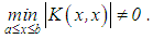 Then, for a regularized framework
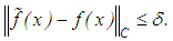
 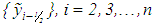 satisfying equation (29), the following estimate in respect of the error of the approximate solution is valid:
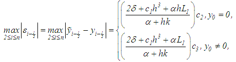 | (30) |
where 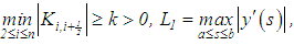
 Let us analyze the estimate in equation (29). The first component on the right-hand side
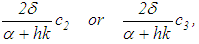 | (31) |
characterizes the influence on the exact regularized framework by the right-hand side error. The second component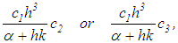 is connected with the approximation of the quadrature integral, while the third component
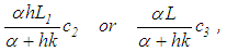 reflects the contribution of the total error of distortion of the desired equation (28) due to the additional
  -component.It is seen that the error estimate in equation (29) unites the h–regularization estimate. This can be observed in equation (23) with the Denisov’s
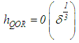
  -regularization estimate in equation (25).We call the quasi-optimal regularizer (QOR) of the parameters
  and h, the minimizer of the right-hand side of equation (29). This implies
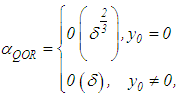 | (32) |
 | (33) |
and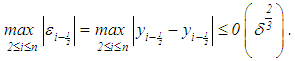 | (34) |
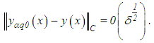
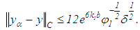
Since, in practice, it is not clear which of the cases results in  or
or  , it is, therefore, good to select one of the relationships in the equation (32) for the asymptote
  but maintaining the condition in equation (32). Indeed, if we set
 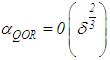 , then
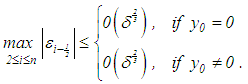 | (35) |
If we set  , then
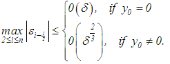 | (36) |
In all cases, however, 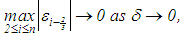 irrespective of whether
  or
or  , that is, the algorithm obtained from solving the system of linear algebraic equation (28) and also equation (22) taking advantage of asymptotes (32) and (33) are regularized. Besides, unlike Denisov’s, the method does not use the
  component, and the requirement of
  or
or  is compensated by changing the dependence of the quasi-optimal asymptote
  and
and  Finally, we note that as long as
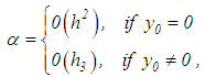 then as
  ,
,  decreases faster than h (the carrier of the basic stability load) and so, parameters h and
  share homogeneous characterizations. As it now stands, the step size h should be regarded as the basic parameter while
  plays the role of the auxiliary. This is reflected by the fact that the presence or absence of
  does not influence the state of the asymptote
  This being so, as soon as
 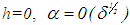 , the
, the  -smoothing equation quickly requires the presence of the component
  ; whereas, when h ≠ 0,
  or
or  , the asymptote
  is such that it replaces the function of
  and continues to support the method of regularization without the introduction of the component
  in the desired equation. However, the use of the parameter
  in place of h increases the effectiveness of the method since, for a small h (not to mention when h→0), the error of the solution is notably compressed.
3.5. Sergeev’s Regularization Method
Consider Volterra integral equation of the first kind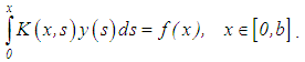 | (37) |
Let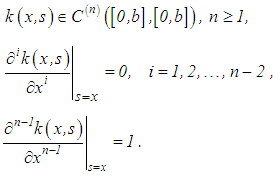 | (38) |
If 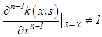 and
and  , we can divide both sides of equation (37) by
 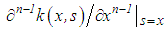 to obtain an equation with property (38).Now, let the function
  be continuous with respect to x and s. Let
 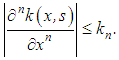 Then after the nth differentiation of equation (37), we obtain a second kind equation
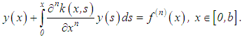 | (39) |
If  Then equation (39) has a unique solution
  (by virtue of the given exact data). But, previously, it was assumed that
  However, if f(x) together with the error is known, then the determination of the derivative f(n)(x) becomes an ill-posed problem and, hence, requires the use of any of the regularization methods. In the studies by Lavrent’ev et al and Sergeev ([15], [16]), a regularization method which also transforms the equation into a second kind equation but does not require the calculation of the said derivative of f(x) without losing the Volterra structure is proposed.Suppose the values
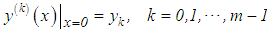 , are known. We introduce the function
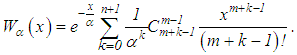 | (40) |
For this equation, let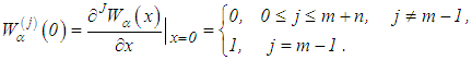 Let it be assumed that in place of the exact right – hand member f(x), the approximate right – hand member
  is known such that
  .Therefore, in place of the exact equation (37) or formally, its equivalent equation (39), we propose the solution of the following approximate Volterra equation of the second kind:
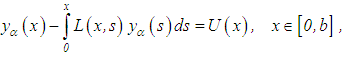 | (41) |
where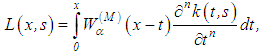
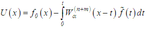 and
and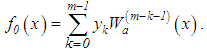 The estimate
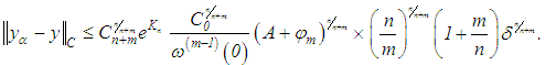
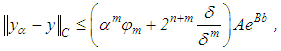 | (42) |
where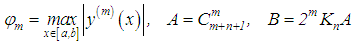 ,is valid. The minimum value of the right-hand side of equation (42) is obtained if
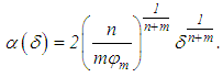 | (43) |
For such value of  ,
,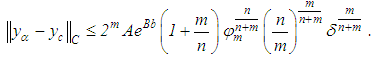 | (44) |
It is clear that 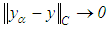 as
as  , and what is more,
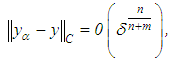 | (45) |
that is, the algorithm obtained from equation (41) is regularizing.In what appears to be the simplest case, where n = m = 1, it is expected to solve the equation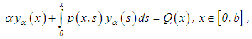 | (46) |
where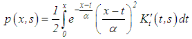 and
and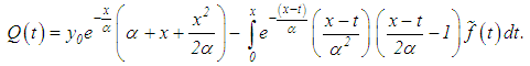 Consequently, we have that
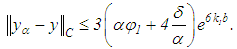 | (47) |
The minimum value of the right-hand side of equation (47) is attained when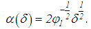 | (48) |
For such  ,
, | (49) |
Here,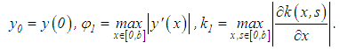
3.6. Magnicki’s Regularization Method
This is closely related to Sergeev’s method but has a wider range of applications. We consider the equation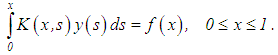 | (50) |
Let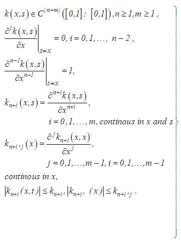 | (51) |
Furthermore, let Then, differentiating equation (50) n times, we obtain the equation
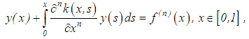 | (52) |
which has a unique solution 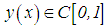 . Again, similar to Sergeev’s method, we assume that
  and that
  are known.Therefore, in place of equation (50) or (52), we propose the solution of a Volterra integral equation of the second kind
 | (53) |
Subject to the conditions:
 a class of functions defined by the following conditions:
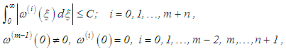 and there exist
  such that
  The following estimate is valid
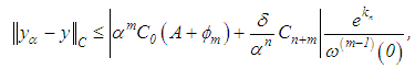 | (54) |
where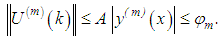 The minimum value of the right-hand side is attained when
 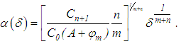 For such values of
 As
As 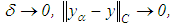 that is, the algorithm obtained from equation (53) is regularizing.For
  ,
, are continuous in x and s,
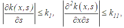 ,we propose a special equation (which is not necessarily a consequence of equation (53)):
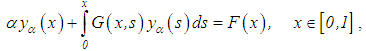 where
where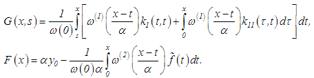 The following estimate (for an optimal value of
  ) is valid:
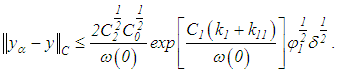 Now, with
  conditions similar to those of equation (51), it becomes necessary to solve the following consequence of equation (51):
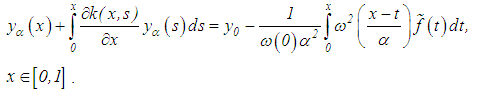 We obtain the following estimates
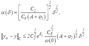
4. Conclusions
Although this study primarily examined regularization methods for first kind Volterra integral equations that maintain the Volterra structure, we never lost sight of the distinguishing features associated with this class of equations, which reflect in the uncertainty and difficulties surrounding their nature when attempting to find their solutions using one or other existing numerical methods. On the other hand, an attempt to solve Volterra integral equations of the first kind using analytic techniques may not be fruitful after all. This is so, because Volterra integral equations of the first kind, in a sense appears to be situated mid-way between Volterra integral equations of the second kind and Fredholm integral equation of the first kind. Precisely, if a Volterra integral equation of the second kind is well-posed and can be effectively solved by any classical means, then a Fredholm integral equation of the first kind is ill-posed, given any preconceived functional space and solvable by special approximating methods. Again, Volterra integral equation of the first kind may be well- posed or ill-posed depending on the choice of the solution space and can only be solved effectively by regularization methods.
References
| [1] | Tikhonov, A. N. and Arsenin, V. Y. (1977). Solutions of ill-posed Problems. Washington; Winston and Sons. |
| [2] | Apartsin, A. C. (1979). On numerical solution to integral equation of the first kind by regularization of quadrature method. Methods of optimization and its application 9; pp. 99-107. |
| [3] | Tikhonov, A. N. & Arsenin, A. A. (1979). Methods of solving ill-posed problems 2nd ed. Mir Publishes. Nauka: p. 288. |
| [4] | Tikhonov, A. N. (1963a). The solution of ill-posed problems, Doklady, Akad. Nauk SSSR, 151, 3. |
| [5] | Savelova, T. I. (1972). On a solution to convolution type equations with non- exact value of the kernel by regularization method. Journal of Applied Mathematics and mathematical Physics, 12, No. 1: pp. 212 – 218. |
| [6] | Savelova, T. I. (1974a). On the application of one clan of regularization algorithms for solving convolution type integral equations of the first kind in Banach Space. Journal of Applied Mathematics and Mathematical Physics, 14, No.2: pp. 479 – 483. |
| [7] | Savelova, T. I. (1974b). Projectional method of solving linear ill- posed problems. Journal of Applied Mathematics and Mathematical Physics 14, No. 4: pp. 1027 – 1031. |
| [8] | Savelova, T. I. (1975a). On regularization of convolution type integral equations of the first kind, Journal of Applied Mathematics and Mathematical Physics, 15, No. 2: pp, 298 – 304. |
| [9] | Savelova, T. I. (1975b). On regularization of system of linear convolution type integral equations of the first kind. Journal of Applied Mathematics and Mathematical Physics, 15, No. 6: pp. 1381 – 1388. |
| [10] | Savelova, T. I. (1978a). About optimal regularization of convolution type equations with Approximate Right-hand Member and Kernel. Journal of Applied Mathematics and Mathematical Physics, 18, No. 1: pp. 218 – 222. |
| [11] | Savelova, T. I. (1978b). About optimal regularization of convolution type equations with sudden charges in the values of the right-hand number and the Kernel. Journal of Applied Mathematics and Mathematical Physics, 18, No. 2: pp. 275 – 283. |
| [12] | Gakhov, F. D. & Cherskii, Ya. I. (1978). Convolution type equations. Mir. Publishes, Nauka: p. 296. |
| [13] | Blondel, J. M. (1971). Phenomene de pertubation singuliere pour une equation integrale lineaire de Volterra. Ibid., 5, No 3: pp. 67 – 72. |
| [14] | Denisov, A. M. (1975). The approximate solution of a volterra equation of the first kind, Journal of Computation Mathematics and Mathematical Phyiscs, 15, No 4: pp. 237 – 239. |
| [15] | Lavrent ev’, M. M., Romanov, V. G. & Shishatskii, S. P. (1980). Ill-posed problems of mathematical physics and analysis. Mir Publishes, Nauka: p. 288. |
| [16] | Sergeev, V. O. (1971). Regularization of Volterra’s Equations of the First Kind. DAN SSSR, 197, No. 3: pp. 531 – 534. |

 Abstract
 Reference
 Full-Text PDF
 Full-text HTML