1. Introduction

Consider Neumann type two-sector model [1] that is denoted as . Let’s introduce the denotations:

base funds of the sector;

number of the labor in the sector;

consumption fund of the sector;

specific consumption (wage rate) in the sector;

national income in the sector;

capital-labor force ratio in the sector,

ratio of fixed assets disposals in the sector;

production function of the sector. Sometimes instead of the function we’ll consider the function

It is expected that the total labor force is In paper [2] the dependence of the consumption volume on the labor force is investigated. In this paper the following problem is set: to distribute the labor between the sectors such that to maximize the total consumption. At the same time as a production function the function with constant elasticity of substitution (CES) is considered [1, 3, 4, 6, 8].

2. Main Part

So, consider the problem of maximizing the total consumption

(1)

under the condition

(2)

Here is a consumption fund in the sector, under the assumption that the special consumption is chosen by the formula

(3)

where is the unique root of the equation

(4)

Since may be expressed as function of

(5)

where and are defined by the equalities

then the following relations are valid

(6)

where is an inverse to function defined by the formula (5).

Now suppose that as a production function will be considered the function with a constant elasticity of substitution (CES)

(7)

where

It is proved that [2] in the case when is a production function with a constant elasticity of substitution (CES) the consumption computed by the formula (6), reaches its maximum in some point and is a unique local extremum point, the function has the only inflection point which changes the concavity to the convexity while

Note that capital-labor ratio in which the maximum of the consumption function of the defined by the formula (6) is reached is the same at all times. Therefore, the point depends only on the national wealth

(8)

where

Suppose that (3) has a unique solution and is a point in which the function reaches its maximum. As above and are found from the conditions

Here we give

Lemma 1. Let the following conditions be fulfilled

а)

b) for some moment .

Then

Proof. Let and . Since and are increasing functions and

then and therefore Since we have Considering (8) we get

Lemma is proved.

Note. It is easy to check that the condition is satisfied if

Let’s show this. The points and are solutions of the equations

where Then

Let

Note that the functions and are increasing and - decreasing and moreover

and

It follows from the last that the equation has a unique solution if and only if, when that is equivalent to the inequality

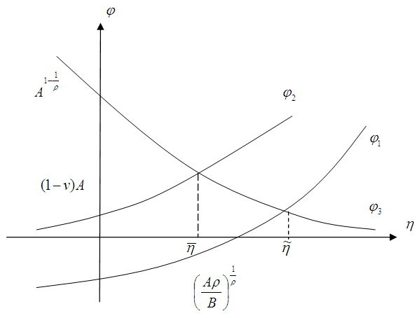
Then if and only if when Due to the properties of and we have (Fig.1).

Figure 1

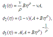
Therefore the inequality is satisfied if

(9)

Let’s calculate and

As follows from (9)

From this we obtain

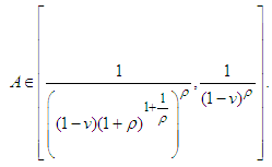
Consequently, for the fulfillment of the condition а) of Lemma 1 it is enough to take from the interval

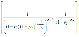
Let and

It is valid

Theorem 1. Let the conditions

а)

b)

be satisfied. Then for all and moreover decreases.

Proof. First we show that Actually, from the condition and (8) follows that Since the total number of the labor is equal to unit, the function is increasing and concave on the interval . Considering that we obtain from the last that increases on the interval and decreases on . Therefore the solution of problem (1) lies on the interval It gives

Suppose that Then from the second condition of b) follows that This means that If then and then

From we get

Thus Besides in the proof was shown that and so considering we get

Now using Lemma 1 we obtain

From this considering after the similar considerations may be shown that and

Continuing this process we arrive at the proof of the theorem.

3. Consequence

If the conditions of Theorem 1 are satisfied then and total consumption

tends to .

Assume that the potential of the second sector is higher than the first sector. Then Theorem 1 is an example of the fact that under certain assumptions in the problem of maximization of the total consumption in contrast to the problems with the same wage rates we do not observe the replacement of the labor force to the second, more "better" production [2]. Moreover, in fact, the labor force in the second sector is upper bounded by the decreasing sequence. Also limit the total consumption is less than the similar limit in the problem with the same wages.