-
Paper Information
- Previous Paper
- Paper Submission
-
Journal Information
- About This Journal
- Editorial Board
- Current Issue
- Archive
- Author Guidelines
- Contact Us
Applied Mathematics
p-ISSN: 2163-1409 e-ISSN: 2163-1425
2017; 7(1): 5-13
doi:10.5923/j.am.20170701.02

Hepatitis B Optimal Control Model with Vertical Transmission
 Abstract
 Reference
 Full-Text PDF
 Full-text HTML
Sacrifice Nana-Kyere1, Joseph Ackora-Prah2, Eric Okyere3, Seth Marmah4, Tuah Afram5
1Department of Mathematics, Ola Girl’s Senior High School, Kenyasi, Ghana
2Department of Mathematics, Kwame Nkrumah University of Science and Technology, Kumasi, Ghana
3Department of Basic Sciences, University of Health and Allied Sciences, Ho, Ghana
4Department Name of Mathematics, Methodist Senior High School, Berekum, Ghana
5Department of Mathematics, Sunyani Senior High School, Sunyani, Ghana
Correspondence to: Sacrifice Nana-Kyere, Department of Mathematics, Ola Girl’s Senior High School, Kenyasi, Ghana.
| Email: |  |
Copyright © 2017 Scientific & Academic Publishing. All Rights Reserved.
This work is licensed under the Creative Commons Attribution International License (CC BY).
http://creativecommons.org/licenses/by/4.0/

The paper presents a model for the transmission dynamics of hepatitis B disease with vertical transmission incidence. The model is investigated using the tool of dynamical system, which reveals the spreading of the epidemic, when the threshold parameter: The basic reproduction number exceeds one. The model is modified by reformulating as an optimal control problem to assess the effectiveness and impact of treatment on the infective. The optimality is deduced and solved numerically to investigate the cost effective control efforts in reducing the number of exposed and infective.
Keywords: Hepatitis B virus (HBV), Lagrangian, Hamiltonain, Boundary conditions
Cite this paper: Sacrifice Nana-Kyere, Joseph Ackora-Prah, Eric Okyere, Seth Marmah, Tuah Afram, Hepatitis B Optimal Control Model with Vertical Transmission, Applied Mathematics, Vol. 7 No. 1, 2017, pp. 5-13. doi: 10.5923/j.am.20170701.02.
Article Outline
1. Introduction
- Disease modeling has been a tool that has led governments, public health organizations and societies out of spiritual mysticism with regards to causes and transmission of infectious diseases [1].The application of mathematics to the modeling of infectious disease has been the platform where unexplained questions of an epidemic outbreak into a population, its transmission dynamics, the likelihood of the epidemic spreading or dying out in the population of susceptible, the best vaccination strategy that would be efficacious to be embarked on by governments and any treatment possibility of the disease are investigated [2].The world health organization (WHO, 2016) reported that, Hepatitis B, is a potential life-threatening liver infection caused by the hepatitis B virus (HBV), an enveloped DNA virus that infects the liver and causes hepatocellular necrosis and inflammation. The disease is transmitted by means of exposure to the blood of infected person and various body fluids; saliva, menstral, vaginal and seminal fluid. The disease is also spread sexually in unvaccinated gay men and persons with several sex partners. Furthermore, in highly endemic areas, HBV is transmitted from mother to child at birth from contact with maternal blood and secretions at delivery.There have been estimated 8 million cases of HBV infection, 240 million chronic carriers and 686,000 deaths globally every year. These estimates render viral hepatitis B to be ranked among the most virulent diseases in the world [3].Concerning hepatitis B disease, several contributions from mathematical models with deep revelations on transmission dynamics and control intervention decision making have been made. Anderson and May [4], proposed a simple mathematical model that explains the effect of carriers on the transmission of HBV. Zou et al [5], used a mathematical model to examine the transmission dynamics as well as the prevalence of HBV in mainland China. Reza et al [6], studied the dynamics of hepatitis B virus (HBV) infection under administration of a vaccine and treatment with both vertical and horizontal transmission. Eikenbery et al [7], analyzed the dynamics of a model using logistic hepatocyte growth and a standard incidence function governing viral infection. The model also considered an explicit time delays in viral infection. Sacrifice et al [8], formulated a simple SITR treatment model of hepatitis of type B. The model investigated the effect of treatment on the infectives in the treated compartment.Notwithstanding, optimal control models have been used extensively in identifying the therapeutic strategies that could be used to eradicate or minimize the disease at a minimal cost [9-13]. Forde et al [14], investigated an optimal control problem for a delay differential equation model of immune responses to hepatitis virus B infection. The model investigated the interplay between virological and immunomodulatory effects of therapy, control of viremia and administration of the minimal dosage in a short time frame. Ntaganda [15], used direct approach and Pontryagin’s maximum principle to solve a hepatitis B virus dynamics optimal control problem. Armbruster and Brandeau [16], developed a mathematical model of a chronic treatable infectious disease and used it to assess the cost and effectiveness of different levels of screening and contact tracing. The model determines the optimal cost-effective equilibrium level of the disease. Hettaf [17], analyzed the optimal efficiency of drug therapy in inhibiting viral protection and preventing new infections. Ntaganda and Gahamanyi [18], presented a fuzzy logic approach to solve a hepatitis B virus Optimal control problem. Elaiw et al [19], considered a nonlinear control system with control input defined to be dependent on the drug dose and drug efficiency. However, treatment schedules for HBV infected patients was developed by using multirate predictive control (mpc). Bhattacharyya and Ghosh [20], studied optimal control of vertically transmitted disease of HBV with regards to its computational and mathematical methods in medicine.Entrenched in all these mathematical models, backed up by the optimal control models of the viral hepatitis B are the devotees of the achievements of the insightful explanations on the transmission dynamics, therapeutic strategies that could be adopted to enhance the treatment of the disease and the control preventive strategy that could be administered to prevent an invading of epidemic. Yet, none of these works can be completely exhibit all that is observed clinically as well as accounting for the full course of the infection.In this research article, we consider a basic model for hepatitis B viral infection that includes a fraction of the offspring of the infected and exposed individuals infected with the disease at birth, and hence enter the exposed compartment, giving vertical transmission of the disease as studied in section 2. The model estimates one imperative qualitative threshold parameter, the basic reproduction number. The section 3 formulates an optimal control problem that minimizes the number of exposed and infective and the cost of treatment of the infected persons by incorporating time dependent control functions. The necessary conditions for an optimal and the corresponding states are then derived by employing the Pontryagin’s Maximum Principle. Finally, in section 4, the resulting optimality system is numerically solved and interpreted from the epidemiological point of view.
2. Model Framework
- In this section, viral hepatitis B transmission epidemic model in a constant population where natural birth rate equals death rate
 is presented. The population at time
  is categorized into the populations of susceptible,
  Exposed,
  Infective,
  and Removed,
  The exposed individual becomes infected with a constant rate
  and infected individuals recover with rate
  is assumed to be the contact rate between the susceptible and the infective. The model assumes that a fraction of the offspring of the exposed and infected individuals are infected with the disease at birth and so enters the exposed compartment, giving vertical transmission of the disease. Thus a fraction
  of the offspring from the exposed individuals and a fraction
  of the offspring from the infective individuals are born into the exposed class. The model is a version of the model proposed by [24]. The compartmental mathematical model is represented by the following system of four differential equations:
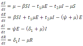 | (1) |
 | (2) |
2.1. The Basic Reproduction Ratio and the Stability of the Disease-free equilibrium
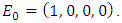
- There exist a unique disease-free equilibrium (DFE) of hepatitis model (1) and is given by
 The basic reproduction number,
  is deduced by the next generation matrix [2]. This is given by
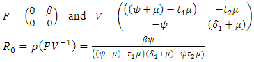 | (3) |
 and unstable if
3. Optimal Control Strategies
- In system (1), we modified the transmission rate by reducing the factor by
 where
where  measures the effort to reduce the contact between the susceptible and the infective individuals. The control variable
  represents the rate at which infected individuals are treated at each time. We further assume that
  individuals at any time
  are removed from the infective class and added to the removed class. With regards to these assumptions, the dynamics of system (1) are modified into the following system of equations:
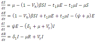 | (4) |
 | (5) |
 and
and  respectively. The quantities
  and
and  denote the weight constants of the exposed and infective human population. Also, the quantities
  and
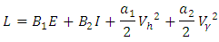
and  are weight constant for reducing the number of exposed and infective and treatment of infective. The term
  and
and  represent the cost associated with the reduction in the exposed and infective and treatment of infective. The cost associated with treatment could be offering the hepatitis B infected person with drugs such as Tenofovir.Here, we seek to find a control functions such that
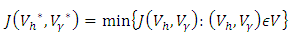 | (6) |
 | (7) |
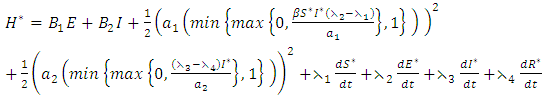
 Here, we seek the minimal value of the Lagrangian. This is done by defining the Hamiltonian H for the control problem as
 | (8) |
3.1. Existence of Control Problem
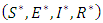
- For the existence of the optimal control problem, we state and prove the following theorem.Theorem 3.1: There exists an optimal control

 such that
 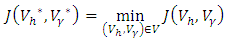 Subject to the control system (4) with the initial conditions (2)Proof: corollary 4.1 of [21] gives the existence of an optimal control due to the convexity of the integrand of
  with respect to
  a priori boundedness of the solutions of both the state and adjoint equations and the Lipchitz property of the state system with respect to the state variables.To find the optimal solution, we apply Pontryagin’s maximum principle [22] to the Hamiltonian (8), such that if
  is an optimal solution of an optimal control problem, then there exists a non trivial vector function
 which satisfies the inequalities
 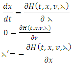 | (9) |
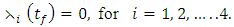
 are optimal state solutions and
  are associated optimal control variables for the optimal control problem (4)-(5), then, there exist adjoint variables
  for
for  satisfying
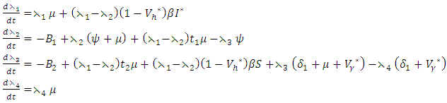 | (10) |
 | (11) |
 | (12) |
 | (13) |
 , and
, and  and differentiating the Hamiltonian (8) with respect to
  and
and  respectively gives equation (8). By solving the equations
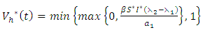
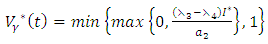
 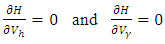 On the interior of the control set and using the optimality conditions and the property of the control space V, we obtain equations (12)-(13).Further, we infer from equation (12)-(13) for
 the characterization of the optimal control. The optimal control and the state variables are found by solving the optimality system, which includes the state system (4), the adjoint system (10), the boundary conditions (11), and the characterization of the optimal control (12)- (13). Thus the optimality system is solved by the use of the boundary conditions together with the characterization of the optimal control
  given by (12)-(13).Furthermore, the second derivative of the Langrangian with respect to
  and
and  are positive, which implies, the optimal problem is minimum at controls
  Hence, substituting the values of
  and
and  in the control system (4) gives
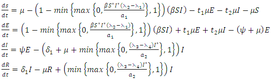 | (14) |
 at
at 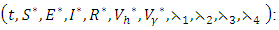
 | (15) |
4. Numerical Results and Discussion
- Here, we numerically investigate the effect of the optimal control strategies on the transmission dynamics of hepatitis B epidemic model with vertical transmission. The optimal control is obtained by solving the optimality system; state system and adjoint system. We then apply an iterative scheme in solving the optimality system. First, we solve the state systems of equations with a guess for the controls over the simulated time frame using fourth order Runge-Kutta scheme. Due to the boundary conditions (11), the adjoint system is solved by backwards fourth order Runge-Kutta by employing the current iterative solutions of the state equation. The controls are then updated by means of a convex combination of the previous controls as well as the characterizations (12) and (13). The whole process is repeated until the values of the unknowns at the previous iterations are closed to the one at the current iterations [23].The model investigates the transmission dynamics of Hepatitis B virus with vertical transmission incidence. We study the control effects of prevention of the interaction between the susceptible and the infectives and treatment control on the spread of the disease. We investigate the effects of the control strategies by comparing numerically the results of the stated scenarios with simulated values taken from [20]:
 and
and  with the initial condition


 Here, we assume that the wight factor,
  associated with control
  is greater than
  and
and  respectively, which are association of control
  This is due to the fact that the cost of implementing
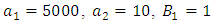
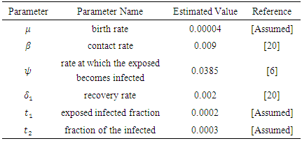
  includes, the cost of screening and surveillance and educational campaign of educating the public against such practices of receiving blood from untested individuals and the need to avoid if possible, becoming exposed to various bodily fluids of infected persons and the need of pregnant women having safe sex with outsiders and even long term partners. The cost of treatment includes hospitalization, medical examination and the administration of antiviral drugs for Hepatitis B. Here, we illustrate the effect of various optimal control strategies on the spread of Hepatitis B epidemic model in an endemic population. The parameter values used in the simulations are estimated based on a Hepatitis B disease as given in Table 1. Other parameters were chosen arbitrary for the numerical simulation.
|
 without and with controls for different values of
  In the absence of control, the susceptible (solid curve) decreases sharply in the first ten years until all the susceptible population are infected with the disease and leaves no population of susceptible. In the presence of controls, the susceptible (dashed curve) decreases slowly, and their population are maintained until about thirty five years where all their population degenerated due to being infected.
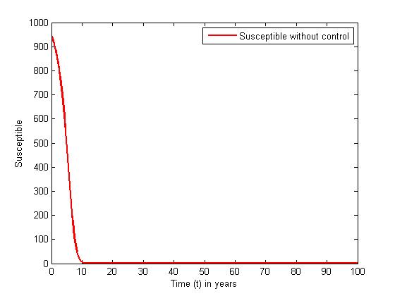 | Figure 1. The plot represents population of susceptible individuals without control |
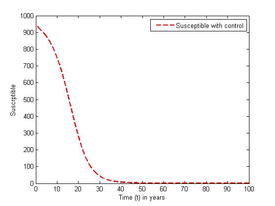 | Figure 2. The plot represents population of susceptible individuals with control |
 without and with controls for different values of
  When there are no controls, the exposed (solid curve) increases sharply in the first nine years, and decreases sharply for the rest of the years. In the presence of control, the number E (dashed curve) increases gradually in the first twenty years and decreases slowly for the rest of the years.
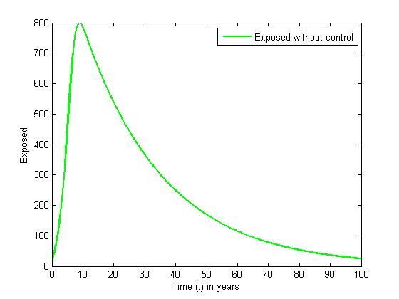 | Figure 3. The plot represents population of Exposed individuals without control |
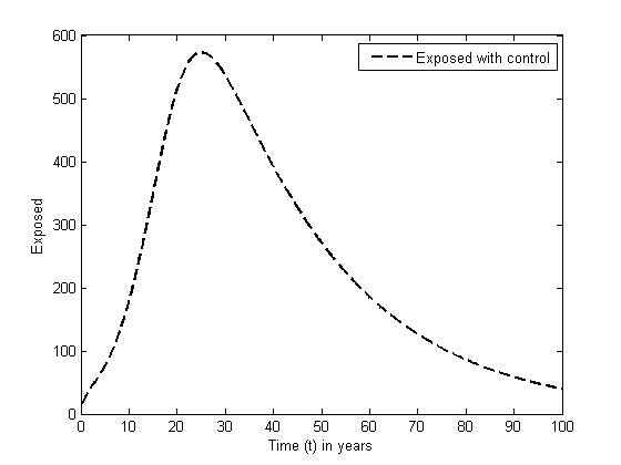 | Figure 4. The plot represents population of Exposed with control |
 without and with controls for a set of values of
  In the absence of control, the infective (solid curve) increases highly and maintains its equilibrium for the rest of the years. The presence of control resulted in the number of infective (dashed line) increased in the first twenty month. However, the control strategy proposed was effective in minimizing the infective population drastically.
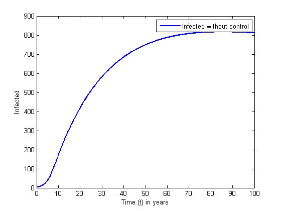 | Figure 5. The plot represents population of Infected individuals without control |
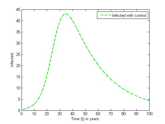 | Figure 6. The plot represents population of Infected individuals with control |
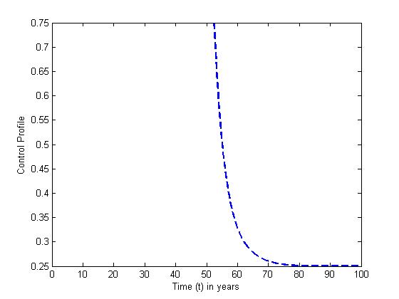
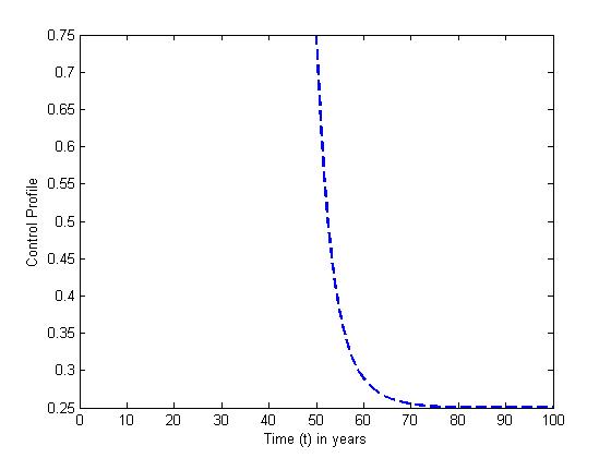
 and the treatment control
  for
for  We see that the preventive control
  is at the upper bound till
  when it slowly drops to the lower bound, while the optimal treatment
  is at the peak of 100% for
  before is drops sharply to the lower bound at
  This implies that least effort would be required in employing the strategy of treatment of the infected individuals for
 | Figure 7. The plot represents optimal control  with with  |
 | Figure 8. The plot represents optimal control  with with  |
 and the treatment control
  are presented for
  The plots show that the preventive control is at the upper bound for
  when it gradually ebb off to the lower bound. The treatment control
  however stayed at the upper bound for
  till it drops to the lower bound. This also suggest that a smaller effort is need ed for treatment of infected individual than the prevention of the susceptible from becoming infected when
 | Figure 9. The plot represents Optimal control  with with  |
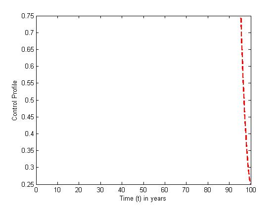 | Figure 10. The plot represents Optimal control  with with  |
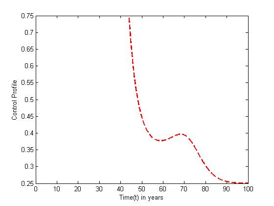
 and the treatment control
  for
for  Here, we notice that the preventive control
  is at the upper bound till
  before it ebbs away gradually to the lower bound at
  while the optimal treatment
  maintains the maximum of 100% for
  when it drops slowly to the lower bound at
  This suggest that a minimal effort is required for the prevention of the disease than treatment under
 | Figure 11. The plot represents Optimal control  with with  |
 | Figure 12. The plot represents Optimal control  with with  |
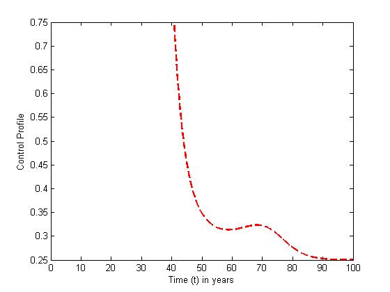
 The optimal control plots indicate that the preventive control
  is at the upper bound till
  when it slowly falls to the lower bound at
  The optimal treatment
  however drops from the upper bound when
  was at 41 and moves gradually to the lower bound at
  This also suggest a requirement of a smaller effort for the prevention of the disease than treatment when
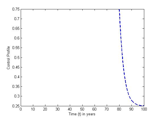 | Figure 13. The plot represents Optimal control  with with  |
 | Figure 14. The plot represents Optimal control  with with  |
5. Conclusions
- In this paper, we formulated and studied the transmission dynamics of hepatitis B disease that employs preventive and treatment controls for optimal control analysis of the model. The necessary conditions for the optimal control of the disease was derived and analyzed. Two types of control functions associated with the reduction of the exposed and the infective and treatment of infective strategies were considered. The control plots that were plotted showed that the number of exposed and infected human decreased in the optimality system. The control analysis indicates that the optimal control strategies have an incomparable effect for the reduction of the infected individuals as compared to the model without control as shown in the plot of figures for the models with control and without control. The simulation results showed that despite the vertical transmission incidence, the proposed control strategy is effective in the reduction of the number of the infective of the disease.