Sacrifice Nana-Kyere1, Seth N. Marmah2, Tuah Afram3, Ernest Owusu-Anane4
1Department of Mathematics, Ola Girl’s Senior High School, Kenyasi, Ghana
2Department of Mathematics, Methodist Senior High, Technical School, Berekum, Ghana
3Department of Mathematics, Sunyani Senior High School, Sunyani, Ghana
4Department Marketing, Procurement and Supply Chain Management, University College of Management Studies, Kumasi, Ghana
Correspondence to: Sacrifice Nana-Kyere, Department of Mathematics, Ola Girl’s Senior High School, Kenyasi, Ghana.
| Email: |  |
Copyright © 2016 Scientific & Academic Publishing. All Rights Reserved.
This work is licensed under the Creative Commons Attribution International License (CC BY).
http://creativecommons.org/licenses/by/4.0/

Abstract
The modeling of infectious disease has been a means of study of disease spread and predicting of an outbreak as well as evaluating strategies for the control of the epidemic. Epidemic models are normally classified based on the disease status. In this article, we study SI vaccination model. The threshold parameter R0 is deduced which shows the disease would spread if its value exceeds one. The global stability of the disease-free and the endemic equilibrium is studied by using the theorem of a Lyapunov function. We adopt the stochastic version of the model and analyzed the stability of the stochastic positive equilibrium. Numerical simulation was done for the models which show the population dynamics of the SI models in the different compartments.
Keywords:
Boundedness, Basic Reproduction Ratio, Lyapunov function, Positive equilibrium
Cite this paper: Sacrifice Nana-Kyere, Seth N. Marmah, Tuah Afram, Ernest Owusu-Anane, Nonlinear Analysis of Stochastic SI Vaccination Model, Applied Mathematics, Vol. 6 No. 4, 2016, pp. 78-85. doi: 10.5923/j.am.20160604.03.
1. Introduction
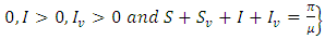
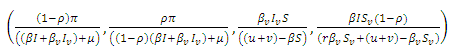
The modeling of communicable diseases with stochastic differential equation (SDE) has gained grounds recently due to its wide range of applications and its ability to reflect reality in epidemiology [3]. Diseases outbreak in a population of susceptibles logically follows stochastic processes, but not the idea of the robustic deterministic as perceived [12]. Stochastic process arises naturally in many physical applications where randomness is to be included in the mathematical model [5, 8]. Stochastic models are adopted when a small number of reacting molecules is present in a modeling system. In such instants of small numbers reacting molecules, fluctuation becomes inevitable and deterministic models become inappropriate to use [2]. In recent years, major studies on stochastic differential equations (SDEs) that have been published by researchers have identified the growing importance of investigating the stability of stochastic positive equilibrium, as well as the global stability of the disease-free and the endemic equilibrium [1, 4, 9].In this paper, we consider the SI vaccination model proposed by Gardon et al. [7] as follows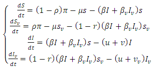 | (1) |
Where  and
and  represent unvaccinated susceptible, vaccinated susceptible, unvaccinated infectives and vaccinated infectives respectively. The model answers one important underlying research subjects; the determination of the existence of the threshold parameter
  which hints on the spreading or dying out of an invading epidemic into a population of susceptible, as studied by various authors [15, 16]. Our motivation lies in the works of Maroufy et al. [14], Adnani et al. [6], Kiouach and Omari [13] and Mukherjee et al [10], who extended their deterministic models to stochastic versions, and studied the stability of the stochastic models. In this research article, we first study the positivity and boundedness of the system (1). The basic reproduction ratio is determined. Applying the hypothetical theorem of the Lyapunov functional, we determine the global stability of the two equilibria for system (1). We extend our stability analysis to the stochastic system (5), which is obtained by random perturbation of the deterministic system (1) and find the stability of its positive equilibrium. Finally, numerical examples which shows the dynamics of systems (1) and (5) are given, which gives the explicit difference in the dynamics of the models.
2. Positivity, Boundedness and Basic Reproduction Ratio
2.1. Positivity and Boundedness
The theory of ordinary differential equations requires that, for every set of initial conditions  the state variables
  of the solution must remain non-negative.Proposition 2.1. Let
  be the solution of the system (1).(a) Given the initial condition
  then there exist a unique positive solution
  for every
  such that the solution will remain in
 with probability of one.(b) The solution
  is defined in the interval
  and
and  where
where 
 Proof: In (a) we let
  Evidently, the coefficients of system (1) are locally Lipschitz continuous. Hence, for any given initial condition
  there exist a unique local solution
  for every
  where
where  is the final time. Here, it can be deduced that
  for every
  Summing the total population of system (1) gives
  Suppose
  is the solution of the differential equation

 where
where  Hence, by comparison theorem;
  as required. Again, we can verify in (b) that
 | (2) |
Integrating inequality (2) gives  for every
  which implies
  It can therefore be verified that the solution
  is bounded within the interval
  This implies
  for every
  Hence
Hence  Hence, employing the same intuition used in proving proposition 2.1, we see that system (1) with non-negative initial conditions
  has a non-negative solution defined in
  and the set
 is invariant by system (1).
2.2. The Basic Reproduction Ratio
The basic reproduction ratio  is defined as an infections originating from an infected individual that invades a population originally of susceptible individuals. Our model calculation would be based on the approach of Diekmann and Heesterbeek ([17]). Here, the functions (F) and (V) denote the rate of new infection term and the rate of transfer into and out of the unvaccinated infectives and vaccinated infectives respectively.The disease compartments are
 Hence
Hence  and
and  The deterministic system (1) has a unique disease-free equilibrium, given by
  where
where  The matrices
  evaluated at
  are given by
 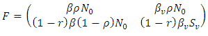 and
and 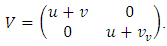 The matrix
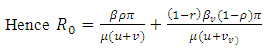
  is a rank one matrix, and its next generation matrix also has rank one ([16]). The spectral radius of a rank one matrix is its trace. Hence
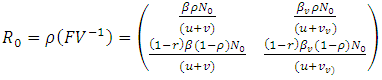
 | (3) |
2.3. Global Stability of the Disease-free Equilibrium
Theorem 2.3: The disease-free equilibrium 
 is globally asymptotically stable in
  whenever
  Proof: We consider the Lyapunov function
 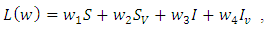 where
where 

 are constants that would be chosen in the course of the proof.Hence, calculating the rate of change of
  along the solution of
  gives,
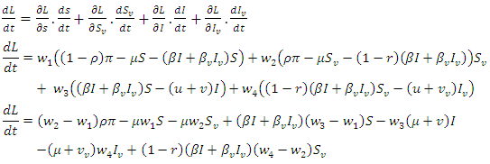 Choosing
  gives the following
  It follows that
  is positive definite and
  is negative definite. It can therefore be ascertained that the function
  is a Lyapunov function for system (1). Hence by Lyapunov asymptotic stability theorem [9], the equilibrium
  is globally asymptotically stable.
2.4. The Global Stability of the Endemic Equilibrium
Theorem 2.4: The unique endemic equilibrium  is globally asymptotically stable in
  whenever
  Proof: We consider the Lyapunovfunction
 are constants to be chosen in the course of the proof. The derivative of
  along the solution of (1) gives
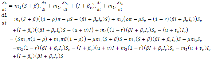 | (4) |
Choosing  and
and  such that
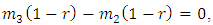 and
and  Then, the relation (4) can be expressed as
 a positive definite and
  is negative definite. Therefore the function
  is a Lyapunov function for system (1) and consequently, by Lyapunov asymptotic stability theorem [13], the equilibrium state
  is globally asymptotically stable. Hence this completes the proof.
3. The Stochastic Model
Here, we introduce stochastic perturbations in the main parameters of the deterministic model (1). Thus we permit stochastic perturbations of the variable  around their values at positive equilibrium
  Hence, we assume that the white noise of the stochastic perturbations of the variable around values of
  are proportional to the distances of
  from
from  Hence the stochastic version of model (1) is
 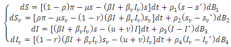 | (5) |
With  where
where  are real constants, and
  are independent wiener processes. We investigate the asymptotic stability behavior of the equilibrium
  of the stochastic equation (5) and compare results with the deterministic model (1).
3.1. Stochastic Stability of the Positive Equilibrium
It can be shown clearly that, the deterministic model (1) has one disease-free equilibrium  which is globally asymptotically stable when
  However, when
  the disease-free equilibrium
  is unstable . Obviously, there is also a unique positive endemic equilibrium
 This equilibrium is globally asymptotically stable. The stochastic system (5) has the same equilibria as the deterministic system (1). Assuming that
  we investigate the stability of the endemic equilibrium
  of (5). The stochastic differential equation (5) can be centered at its positive equilibrium
  by the change of variables
 | (6) |
The linearized system of the stochastic model (5) around  takes the form
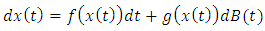 | (7) |
Where  and equals
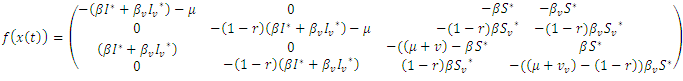
 Clearly, the endemic equilibrium
  corresponds to the trivial solution
  in (7). We denote
  to be the differential operator associated with (7), defined for the family of nonnegative functions
  such that it is continuously differentiable with respect to
  and twice with respect to
  According to Afanas’ ev et al [11], the differential operator
  for a function
  is given by
 | (8) |
Where  and
and  Where
Where  and
and  are the transposition and trace respectively. With reference to Afanas’ ev et al [11], the following results hold.Theorem 3.1: Suppose a function
  exist, satisfying the following inequalities
 | (9) |
Where  and
and  Then the trivial solution of (7) is
  moment exponentially stable. Again, given that
  the trivial solution is said to be exponentially stable in mean square and the equilibrium
  is globally asymptotically stable.From theorem 3.1, the conditions for stochastic asymptotic stability of trivial solution of (7) are given theorem 3.2.Theorem 3.2: Suppose
 and
and  hold, then the zero solution of (7) is asymptotically mean square stable.Proof: We consider the Lyapunov
  With
With 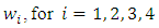 non-negative constants that will be chosen in the course of the proof. It can be easily ascertained that inequality (9) hold true when
  Applying the operator
  on
on  gives
gives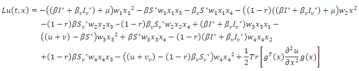 | (10) |
Further | (11) |
Now remark that  and
and 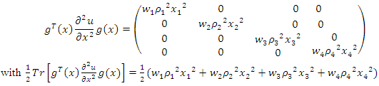 | (12) |
Now, from equation (10), if we choose  and
and  then from equation (10), it is easy to verify that,
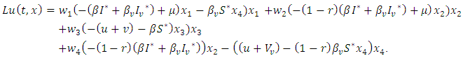 Hence, according to theorem 3.1, the proof is completed.
4. Numerical Examples of the Models
Here, we illustrate with figures the dynamics of the systems (1) and (5), and gives an explicit difference in the models by carrying out numerical simulation for the hypothetical set of parameter values. To demonstrate the differences, we simulate the systems (1) and (5) by using the following set of parameter values; 
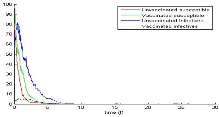
 However, some of the parameters were allowed to change in the course of the simulations in order to bring out the dynamics of the models. The differences in the dynamics of the models are therefore given by the diagrams in the following:Example 1:Here, the dynamic behaviors of the four classes of individuals
  of the deterministic and its stochastic version are plotted against time. Here we assumed the following set of hypothetical parameter values;
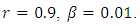 Calculating
  based on theses parameter values gives
  To confirm the deterministic plot of figure1a, we choose white noises
  and
and  of equal strength
  and shows the fluctuations in the trajectories of the plot of the stochastic system (5). We can see that the trajectories of the stochastic plot displayed on our graphs are the same as the trajectories of its deterministic model (1) during a finite time frame.
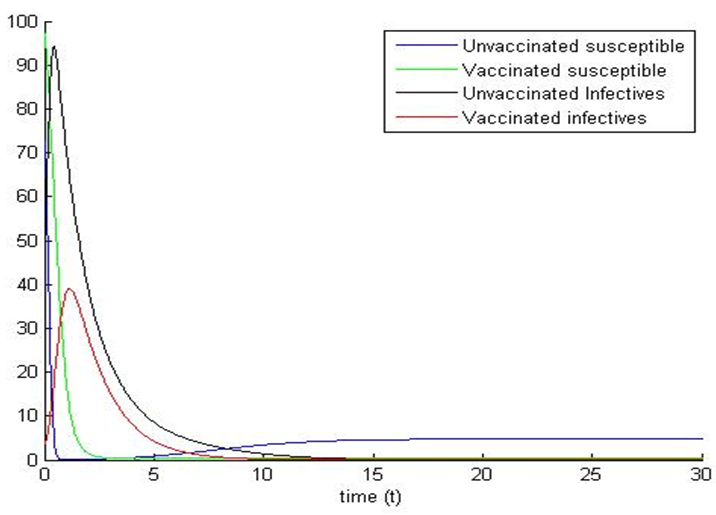 | Figure 1a. |
 | Figure 1b. |
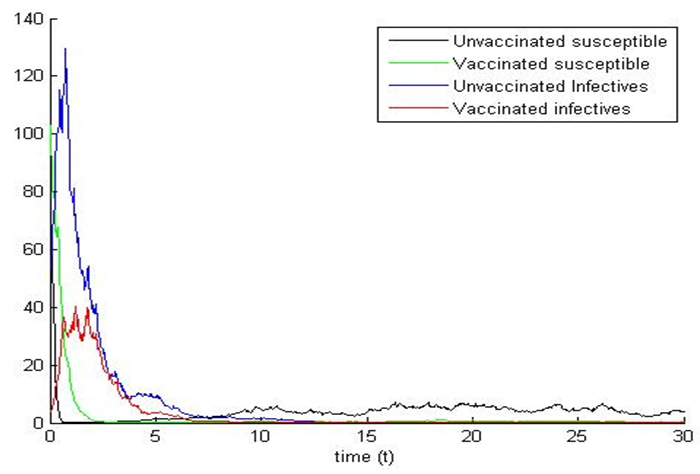
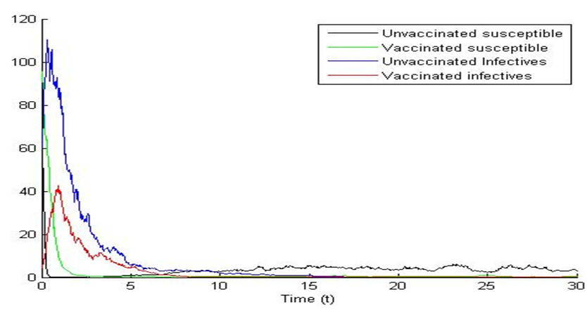
Example 2:Here, we choose the same choice of parameter values: 
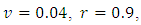 except for
  and the same strength of white noise
 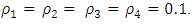 Again, calculating
  on these parameter values gives
  We observe that the path of the trajectories of the systems (1) and (5) are eventually absorbed in the stable point (see figure 1a, 1b, 2a, 2b).
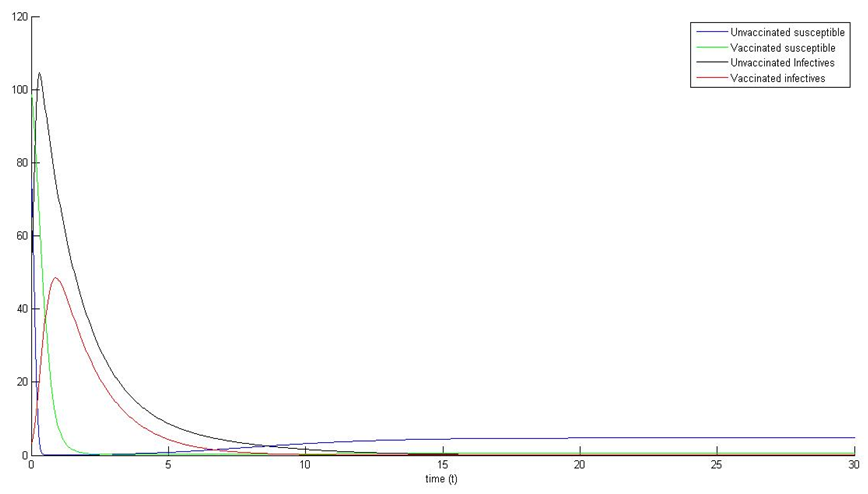 | Figure 2a. |
 | Figure 2b. |
Examples 3Choosing  and
and  we observe that system (1) and (5) are stable (see figures 3a and 3b). Again, the path of the stochastic processes leaves the trajectories and is absorbed in the equilibrium (see figure 3b).
 | Figure 3a. |
 | Figure 3b. |
5. Conclusions
In this paper, the dynamics of deterministic SI vaccination model and its stochastic variant are presented. The stability analyses of the deterministic model were investigated. Suitable Lyapunov functions were constructed for the global stability of the two equilibria. We constructed the stochastic version of the model by employing the idea of Mukhere et al [4, 9, 10].Our main purpose of the study was to investigate the asymptotic stability behavior of the endemic equilibrium  of the stochastic version of the deterministic SI model proposed by Gardon et al [7]. The numerical simulation for the models shows that the trajectories of the stochastic plots were the same as the trajectories of the deterministic model. Further, from our stochastic plots, the simulation shows an initial random fluctuation of the stochastic trajectories, until they eventually approach asymptotic level. We have demonstrated that our stochastic system is globally asymptotically stable in probability when the densities of white noise are less than certain threshold parameters. However, if these densities of white noise are zero, it means there are no stochastic environmental factors on the population and hence no stochastic perturbation. Hence theorem 3.2 conditions would be reduced to the condition
  which implies a nonlinear stability condition for the deterministic system (1). In our future research, we would consider how control strategies may be devised for the model.
References
| [1] | A. Lahrouz, L. Omari and D. Kiouach, ‘‘Global analysis of a deterministic and stochastic nonlinear SIRS epidemic model, 2011, Vol.16, N0.1, 59-76. |
| [2] | F. Brauer, P. Van den Driessche and J. Wu (Eds), ‘‘Mathematical Epidemiology’’, Mathematical Biosciences subseries; 2008, Springer- Verlag Berlin Heidelberg. |
| [3] | C. Damian, ‘‘A Stochastic SIS infection model incorporating Indirect Transmission’’, Journal of Applied Probalility, vol.42, No.3 (sep., 2005), pp 726-737. |
| [4] | P. Das, D. Mukherjee, and Y. H. Hsieh, ‘‘An S-I epidemic model with saturation incidence: discrete and stochastic version’’, International Journal of Nonlinear Analysis and Applications, pp. 1-9, 2011. |
| [5] | X. Q. Liu, S. M. Zhong, B. D. Tian, and F. X. Zheng, ‘‘Asymptotic properties of a stochastic predator-prey model with Crowley-Martin functional response’’, Journal of Applied mathematics and computing, 2013. |
| [6] | J. Adnani, K. Hattaf and N. Yousfi, ‘‘Stability Analysis of a Stochastic SIR Epidemic Model with Specific Nonlinear Incidence Rate, International Journal of Stochastic Analysis, Volume 2013, article ID 431257. |
| [7] | S. Gardon, M. Mackinnon, S. NEE and A. Read, ‘Imperfect vaccination: some epidemiological and evolutionary consequences, Proc. R Soc. Lond. B., 270 (2003), pp. 1129-1136. |
| [8] | F. L. Gregory, Introduction to Stochastic processes, Chapman and Hall, 1995. |
| [9] | D. Mukherjee. Stability analysis of a stochastic model for prey-predator system with disease disease in the prey, Nonli. Anal.; Control 8 (2003), 83-92. |
| [10] | D. Mukherjee, P. Das and D. Kesh, ‘‘Dynamics of a Plant-Herbivore Model with Holling Type II Functional Response’’, Computational and Mathematical Biology, Concept Press Ltd, 2011. |
| [11] | V. N. Afanasev, V. B. Kolmanowski and V. R. Nosov, ‘‘Mathematical Theory of Global Systems Design, Kluwer, Dordrecht, 1996. |
| [12] | M. Carletti, ‘Mean-square stability of a stochastic model for bacteriophage infection with time delays. Math.Biosci. 2007, 210(2): 395-414. |
| [13] | D. Kiouach and L. Omari, ‘‘Stochastic Asymptotic Stability of a SIRS Epidemic Model, European Journal of Scientific Research, ISSN 1450-216X vol.24 (2008), pp575-579. |
| [14] | H. El. Maroufy, A. Lahrouz and PGL Leach, ‘Qualitative Behaviour of a Model of an SIRS Epidemic, International Journal of Applied Mathematics and Information Sciences, 5(2) (2011), 220-238. |
| [15] | C. Castillo-Chavez, Z. Feng and W. Huang, ‘‘On the computation of R0 and its role on global stability, in Mathematical approaches for emerging and reemerging infectious diseases: models, methods and theory, C. Castillo-Chavez, S. Blower, P. van den Driessche, D. Kirschner and A. A. Yakubu,eds., Springer-Verlag, NewYork, 2002, pp.229-250. |
| [16] | P.van den Driessche and J. Watmough, ‘Reproduction numbers and sub-threshold endemic equilibria for compartmental models of disease transmission, Mathematical Biosciences, 180 (1-2), pp. 29-48, November 2002. |
| [17] | O. Diekmann, J. A. P. Heesterbeek, ‘‘Mathematical Epidemiology of infectious diseases: Model building, analysis and interpretation, John Wiley& Sons, New York, (2000). |

 Abstract
 Reference
 Full-Text PDF
 Full-text HTML