-
Paper Information
- Paper Submission
-
Journal Information
- About This Journal
- Editorial Board
- Current Issue
- Archive
- Author Guidelines
- Contact Us
Applied Mathematics
p-ISSN: 2163-1409 e-ISSN: 2163-1425
2016; 6(3): 48-55
doi:10.5923/j.am.20160603.02

Analytical Solutions of Fourth Order Critically Undamped Oscillatory Nonlinear Systems with Pairwise Equal Imaginary Eigenvalues
 Abstract
 Reference
 Full-Text PDF
 Full-text HTML
M. Abul Kawser1, Md. Mahafujur Rahaman2, Mst. Kamrunnaher1
1Department of Mathematics, Islamic University, Kushtia, Bangladesh
2Department of Computer Science & Engineering, Z. H. Sikder University of Science & Technology, Shariatpur, Bangladesh
Correspondence to: Md. Mahafujur Rahaman, Department of Computer Science & Engineering, Z. H. Sikder University of Science & Technology, Shariatpur, Bangladesh.
| Email: |  |
Copyright © 2016 Scientific & Academic Publishing. All Rights Reserved.
This work is licensed under the Creative Commons Attribution International License (CC BY).
http://creativecommons.org/licenses/by/4.0/

In this article, we present asymptotic solutions of fourth order critically oscillatory undamped nonlinear systems in which the four eigenvalues are pairwise equal and imaginary. In this regard, the modified Krylov-Bogoliubov-Mitropolskii (KBM) method is used, which is considered to be a well-suited method for investigating the transient behaviour of oscillating systems, to obtain the solutions of fourth order critically oscillatory nonlinear systems. This paper suggests that the solutions obtained by the modified KBM method are quite well consonant with those obtained by the numerical method using Mathematica.
Keywords: KBM method, Critically oscillatory system, Nonlinearity, Eigenvalues
Cite this paper: M. Abul Kawser, Md. Mahafujur Rahaman, Mst. Kamrunnaher, Analytical Solutions of Fourth Order Critically Undamped Oscillatory Nonlinear Systems with Pairwise Equal Imaginary Eigenvalues, Applied Mathematics, Vol. 6 No. 3, 2016, pp. 48-55. doi: 10.5923/j.am.20160603.02.
Article Outline
1. Introduction
- Generally, a significant approach, known as the expansion of the small parameter, is used to investigate nonlinear oscillatory systems, which is erected upon the perturbation theory. The perturbation theory can be defined as mathematical methods by which an approximate solution to a mathematical problem is figured out. This theory was used as a basis for one of the widely known methods called the Krylov-Bogoliubov-Mitropolskii (KBM) [1, 2] method which is applied to study nonlinear oscillatory and non-oscillatory differential systems with small nonlinearities. In the beginning, this method was developed by Krylov and Bogoliubov [1] to find out the periodic solutions of second order nonlinear differential systems with small nonlinearities. Shortly after that, Popov [3] extended it to damped oscillatory processes. Then, it was expanded further and justified by Bogoliubov and Mitropolskii [2]. However, due to the physical significance of the damped oscillatory systems, Popov's results were rediscovered by Mendelson [4]. Later, the method was extended by Murty and Deekshatulu [5] for over damped nonlinear systems. However, in 1971, Murty [6] propounded a unified KBM method for second order nonlinear systems which covered all the undamped, over-damped and damped oscillatory cases. Next, Osiniskii [7] developed it further and used it to solve third order nonlinear differential systems for the first time, imposing some restrictions on it. But this rendered the solution over-simplified. Therefore, Mulholland [8] lifted those restrictions and found the intended solutions of third order nonlinear systems. Mickens [9] modified the method for nonlinear oscillations with finite damping, and for harmonic oscillations without damping. Bojadziev [10] suggested damped oscillating processes in biological and biochemical systems. Bojadziev and Edwards [11] offered some methods for non-oscillatory and oscillatory processes. Later, Arya and Bojadziev [12] proposed time dependent oscillating systems with damping, slowly varying parameters, and delay. Bojadziv [13] subsequently examined the solutions of nonlinear systems by transforming the method to damped nonlinear oscillations for a 3-dimensional differential system. Then, Alam and Sattar [14] expounded time dependent third-order oscillating systems with damping. Later on, Akbar et al. [15] generalized the method which was less intricate than the method put forward by Murty et al. [16]. Akbar et al. [17] then expanded it for fourth order damped oscillatory systems in the case when the four eigenvalues were complex conjugate. Thereupon, the perturbation solution of fourth order critically damped oscillatory systems was expounded by Haque et al. [18] under the conditions that when two of the eigenvalues are real and equal and the other two are complex conjugate. Later, Rahman et al. [19] presented a technique for fourth order damped oscillatory nonlinear systems in the case when two of the eigenvalues are real and distinct and the other two are complex conjugate.This article provides the solutions of fourth order critically undamped oscillatory nonlinear systems where all the eigenvalues are pairwise equal and imaginary. This paper suggests that the obtained perturbation results are quite well consonant with the numerical results for different sets of initial conditions together with different sets of eigenvalues. In this study, all the results are computed using Mathematica 9.0.
2. Method
- Let us consider a fourth order weakly nonlinear system
 | (1) |
 denotes the fourth derivative and over dots indicate the first, second and third derivatives of
  with respect to time
 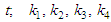 stand for characteristic parameters;
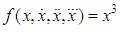
  signifies a positive small parameter and
  is the given nonlinear function. Since the system (1) is of fourth order critically undamped oscillatory, so we consider the equation (1) has pairwise equal imaginary eigenvalues, and assume that the pairwise equal eigenvalues are
  Therefore, the characteristic parameters of equation (1) are defined by
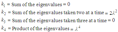 Thus, when
  the solution of the corresponding linear equation of (1) becomes
 | (2) |
 are constants of integration.Nonetheless, if
  following Alam [20], an asymptotic solution of (1) becomes
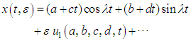 | (3) |
 denote functions of
  and they satisfy the following first order differential equations:
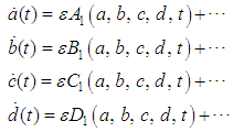 | (4) |
 and
and  for
for  to the extent that
  appearing in equation (3) and equation (4), satisfy the given differential equation (1). In order to determine these unknown functions, it should be noted that, in the KBM method generally the correction terms,
  for
for  exclude the terms, which are also known as ‘secular terms’, that render them larger. Theoretically, the solution can be obtained up to the accuracy of any order of approximation. However, the solution is generally confined to a lower order, usually the first as suggested by Murty [6] owing to the rapidly growing algebraic complexity for the derivation of the formulae.Now, differentiating the equation (3) four times with respect to
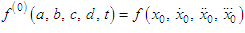
  substituting the value of x and the derivatives
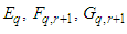
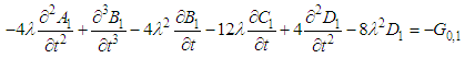
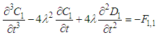
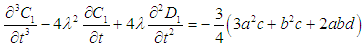
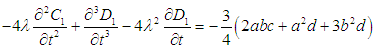
  in the original equation (1), using the relations presented in (4), and, finally, equating the coefficients of
  we get
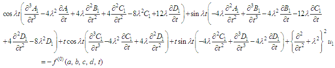 | (5) |
 and
and 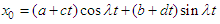 Now, expanding the function
  in the Taylor’s series (see also Sattar [21], Alam [22], Alam and Sattar [23] for details) with respect to the origin in power of
  As a result, we get
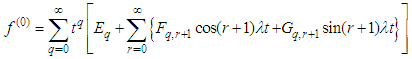 | (6) |
 are functions of
  and
and  are vary from
  but for a particular problem they have some fixed values. Thus, with the help of equation (6), equation (5) becomes
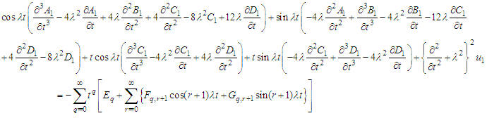 | (7) |
 must not contains the fundamental terms of
  So, equation (7) can be separated for unknown functions
 and
and  as follows:
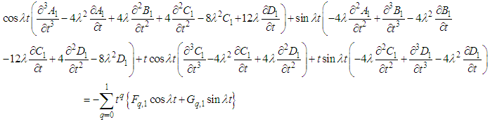 | (8) |
 | (9) |
 and
and  from both sides of equation (8), we get
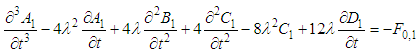 | (10) |
 | (11) |
 | (12) |
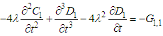 | (13) |
 we have four equations (10) to (13). Therefore, in order to obtain the unknown functions
  we are compelled to use some widely known operator method. From equations (12) and (13) we can determine the unknown functions
  then substitute them into the equations (10) and (11) we can find out the other two unknown functions
  Since
Since  are proportional to the small parameter
  they become slowly varying functions of time
  and, for first approximate solution, we may consider them as constants which are in the right hand side. It should be noted that Murty and Deekshatulu [5], and Murty et al. [16] first made this assumption. Therefore, the solution of the equation (4) becomes
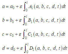 | (14) |
 and
and  in the equation (3), we obtain the complete solution of (1). Thus, the determination of the first approximate solution is complete.
3. Example
- An example has been worked out here using the aforementioned method. Let us consider the Duffing type equation of fourth order nonlinear differential system
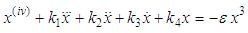 | (15) |
 Thus
Thus 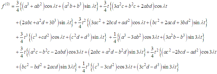 | (16) |
 | (17) |
 | (18) |
 | (19) |
 | (20) |
 | (21) |
 | (22) |
 | (23) |
 and
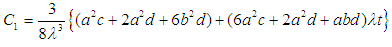
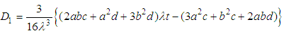
and  from equations (22) and (23) into the equations (18) and (19), and solving them, we get
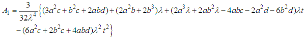 | (24) |
 | (25) |
 | (26) |
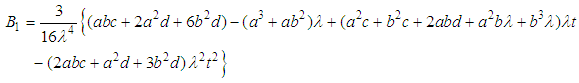
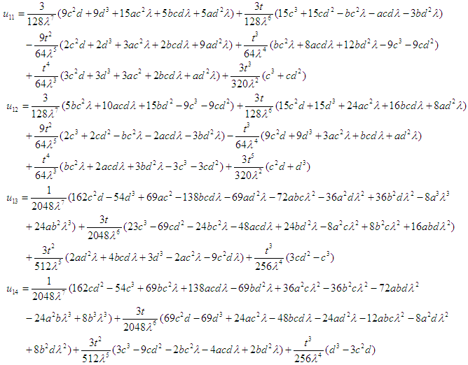 Substituting the values of
  from equations (24), (25), (22) and (23) respectively into equation (4), we get
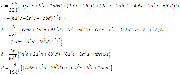 | (27) |
 are proportional to the small parameter
  they are slowly varying functions of time
  It is, therefore, possible to replace
  by their respective values obtained in linear case (i.e., the values of
  obtained when
  ) in the right hand side of equation (27). This type of substitution was first introduced by Murty et al. [16], and Murty and Deekshatulu [5] to solve similar type of nonlinear equations. Thus, the solution of (27) becomes
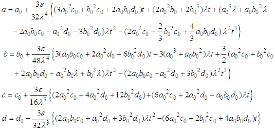 | (28) |
 | (29) |
 are given by the equation (28) and
  is given by (26).
4. Results and Discussion
- In order to test the accuracy of our analytical solution obtained by certain perturbation method, we contrast the perturbation results to the numerical results obtained using Mathematica 9.0 for the different sets of initial conditions. Here,
 is computed by equation (29), where
  are calculated from equation (28); and (26) is used to obtain
  when
when  together with the different sets of initial conditions. We get the results from (29) for different values of
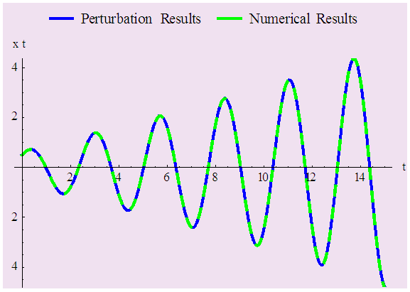
  and figure out the corresponding numerical solution using Mathematica 9.0. Figure 1 to Figure 4 represent all the results, which show the perturbation results and numerical results coincide satisfactorily.
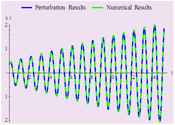 | Figure 1. Comparison between perturbation and numerical results for  and and  with the initial conditions with the initial conditions   |
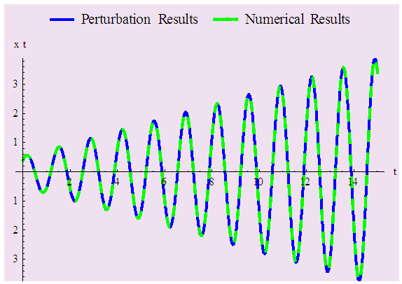
 | Figure 2. Comparison between perturbation and numerical results for  and and  with the initial conditions with the initial conditions  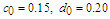 |
 | Figure 3. Comparison between perturbation and numerical results for  and and  with the initial conditions with the initial conditions 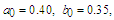  |
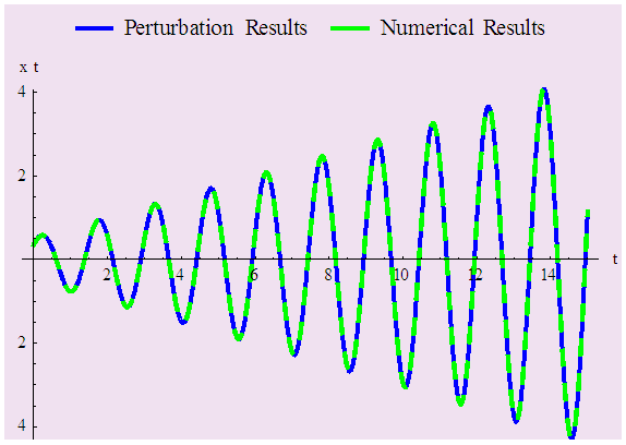 | Figure 4. Comparison between perturbation and numerical results for  and and  with the initial conditions with the initial conditions   |
5. Conclusions
- In conclusion, it can be said that we have modified the Krylov-Bogoliubov-Mitropolskii (KBM) method in this paper, which is regarded as one of the most widely used methods to study the transient behaviour of oscillating systems. Subsequently, we have successfully applied the modified KBM method to the fourth order critically nonlinear oscillatory systems. In relation to the fourth order critically nonlinear oscillatory systems, we have obtained the solutions in such circumstances where in the eigenvalues are pairwise equal and imaginary. It should be noted here that much error generally occurs in the KBM method in the case of rapid changes of x with respect to time t. Nevertheless, all the above figures reveal that, with respect to the different sets of initial conditions, the perturbation solutions of the modified KBM method correspond completely to the numerical solutions. It is, therefore, suggested that the modified KBM method gives highly accurate results which can be applied for different types of nonlinear differential systems.
ACKNOWLEDGEMENTS
- I would like to express my deepest appreciation to Md. Mizanur Rahman, Associate Professor, Department of Mathematics, Islamic University, for his advice and useful comments on the earlier drafts. Special thanks are due to Md. Imamunur Rahman for his assistance.