1. Introduction

Numerous problems in physics, Biology and engineering are modeled by system of differential equations, which are solved by semi-analytical methods like Adomian decomposition method (ADM) [14-15], Homotopy pereturbation method (HPM) [17], New iterative method (NIM) [18], Differential transform method (DTM) [16], Revised new iterative method (RNIM) [19], Taylor collocation mehod (TCM) [21], Variational iteration method (VIM) [20], among others.

Among the above mentioned methods, the RADM is very simple in its principles and applications to solve system of nonlinear differential equations as it does not generate secular terms or rely on trial functions or on a perturbation parameter as other does. Revised ADM [2] was proposed to solve system of ordinary/fractional differential equations. The revised method yields a series solution which converges faster than the series obtained by the standard ADM [14]. This tecnique’s approximation is based on the Adomian polynomial.

Therefore, in this work, we present the application of the RADM to find approximations for a pollution model of lakes system [3-11]. The aim of the model is to describe the pollution of a system of lakes, considering three input models, i.e, periodic (Sinosoidal) input, exponential decaying (Impulse) input and the linear (Step) input as depicted in figure 1. The results obtained are compared with that of DTM, VIM and RK45F method.

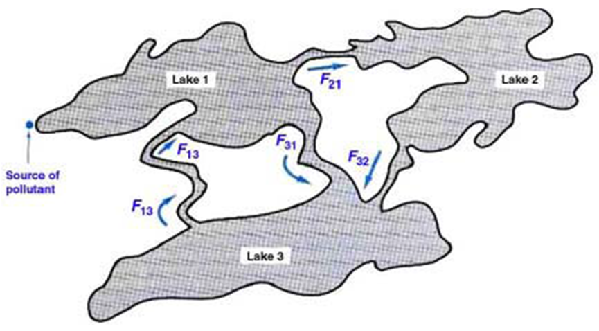Figure 1. System of three lakes with interconnecting channels. A pollutant enters the first lake at the indicated source. [23]

The residual part of the paper is systematized as follows; In section 2, we give a description of the lakes pollution problem. The description on how to apply the RADM to solve system of ordinary differential equations is illustrated in section 3. In section 4, we presented the numerical implementation of the method for the three pollution lakes problems and its numerical results. In section 5, we give a concise discussion of our results. Finally, a conclusion is drawn in the last section.

2. Description of the Model of Pollution Problem

A system of pollution of lakes is a set of lakes interconnected by channels. These lakes are modeled by large compartments interconnected by pipelines [1]. In figure 1, a system of three lakes; and is shown. Arrows represent the direction of flow through each channel or pipeline [22]. When a pollutant enters the first lake, i.e to know the rate of pollutant at which it enters the lake per unit time, is introduced in the system in the system of equations. The function may be a constant or it may vary with time,

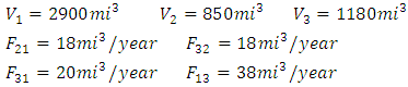
Let the amount of pollution in each lake be denoted by at any time where . It is being assumed that the amount of pollutant is equally distributed in each lake and the volume of each lake remains constant. Also, the type of pollutant remains constant and not transforming into other kinds of pollutant. The, the concentration of the lake is given by

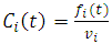(1)

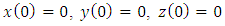
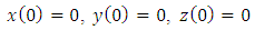
Initially, each lake is considered to be free of pollution, i.e, for So the following conditions are obtained;

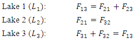Flux of pollutant flowing from lake to lake at any time measures the rate of flow of the concentration of pollutant and is given by

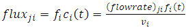(2)

Where is constant from lake to lake It can be easily seen that

(3)

To each lake, we obtain the following system of first order ordinary differential equations:

(4)

with initial conditions

(5)

For results comparison, we consider throughout this paper the values of the parameters (4). [7, 11].

(6)

3. Revised ADM for a System of ODEs

Consider the following system of ordinary differential equations [2];

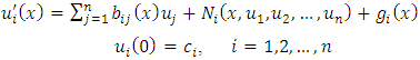(7)

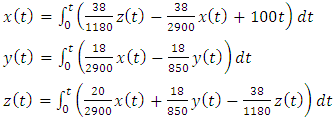
where and are nonlinear continuous functions of its argument. Integrating both side of (7) from to and then, using the initial conditions, we get

(8)

For

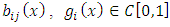
In [2], a modification of the ADM was proposed. There define the following recurrence relation;

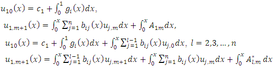(9)

where is defined as

(10)

Here, and are A domain polynomials corresponding to and respectively.

Taking

(11)

4. Numerical Simulation

In this section, we apply the RADM described above to find approximate analytical solutions for the three inputs stated earlier to illustrate the effectiveness and accuracy of the method. To simulate the pollution in the lakes, we coded the RADM in Maple 13.

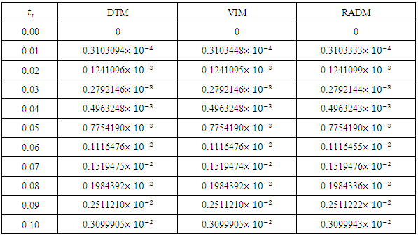
4.1. Periodic (Sinusoidal) Input Model

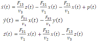
The Sinusoidal input model is used for pollutants that are introduced to the lake periodically. As an illustration, we take where is the average input concentration of pollutant, is the amplitude of fluctuations, and is the frequency of fluctuations. Taking and the parameter values given in (6), the system (4) becomes;

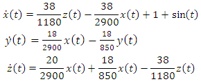(12)

with initial conditions

(13)

The system (12) –(13), is equivalent to the following system of Volterra integral equations of the second kind;

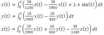The revised Adomian procedure in (9) would lead to

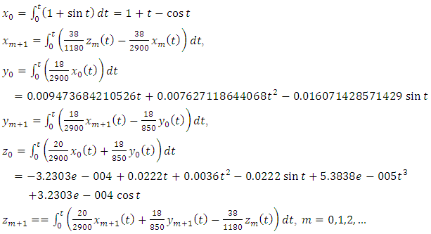The first iteration gives

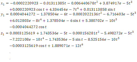After the four iterations, we get

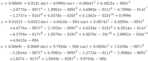
Figure 2. Graphical representation of pollutant dumping periodically in Lake 1, 2 and 3 with RADM and RK45F solutions

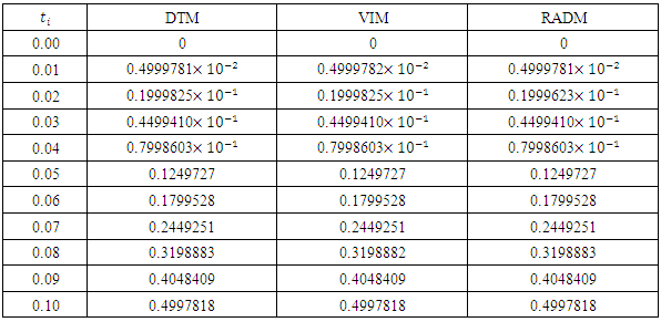
4.2. Linear (Impulse) Input Model

This model describes the steady behavior of the pollutant addition into the lake. At the time zero, the pollutant concentration is also zero but as the time increases the addition of pollutant starts and remains steady afterwards. It can also be understood better by an example [3] that if a manufacturing plant starts production and dump it’s raw wastage on a constant rate, the In this case, Eqn.(9) becomes;

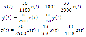(14)

with initial conditions

(15)

The system (14) –(15), is equivalent to the following system of Volterra integral equations of the second kind;

The revised Adomian scheme in (9) would lead to

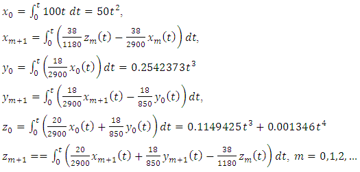The first iteration is

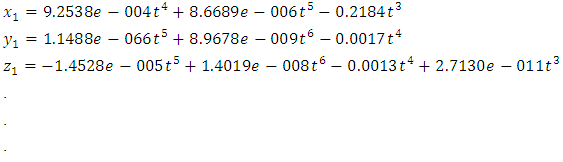And so on. After the third iteration, the sum of the first three iterations is;

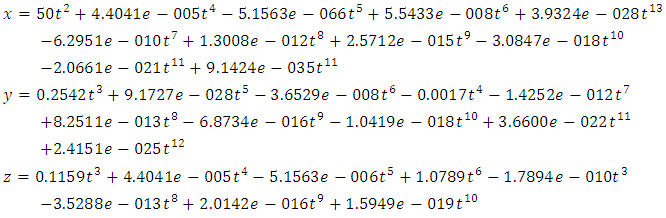
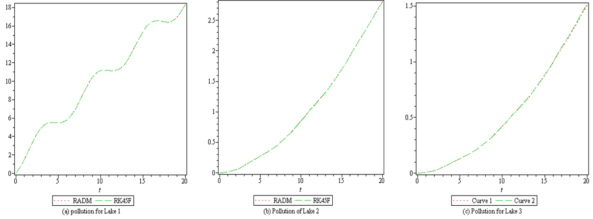
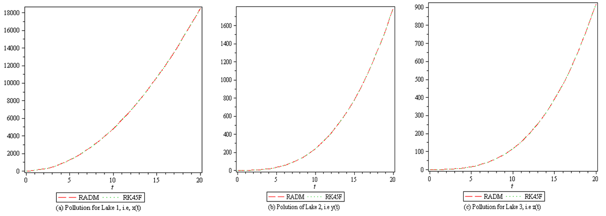Figure 3. Graphical representation of linear input pollutant in Lake 1, 2 and 3 with RADM and RK45F solutions

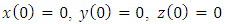
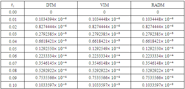
4.3. Exponentially Decaying (Step) Input Model

This model is assumed when heavy dumping of pollutant is under consideration, i.e, 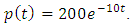For instance, a industry situated in a city collects and store its wastage and dumps it after a few days period. So Eqn.(9) takes the form;

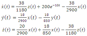(16)

with initial conditions

(17)

The system (16) –(17), is equivalent to the following system of Volterra integral equations of the second kind;

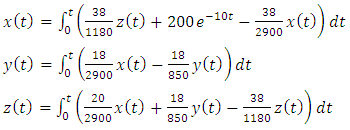The revised Adomian procedure in (9) would lead to

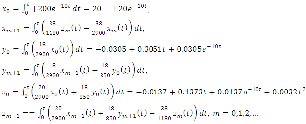The subsequent iteration is

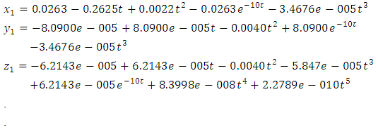The sum of the first three iterations is;

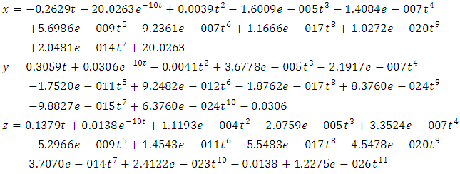
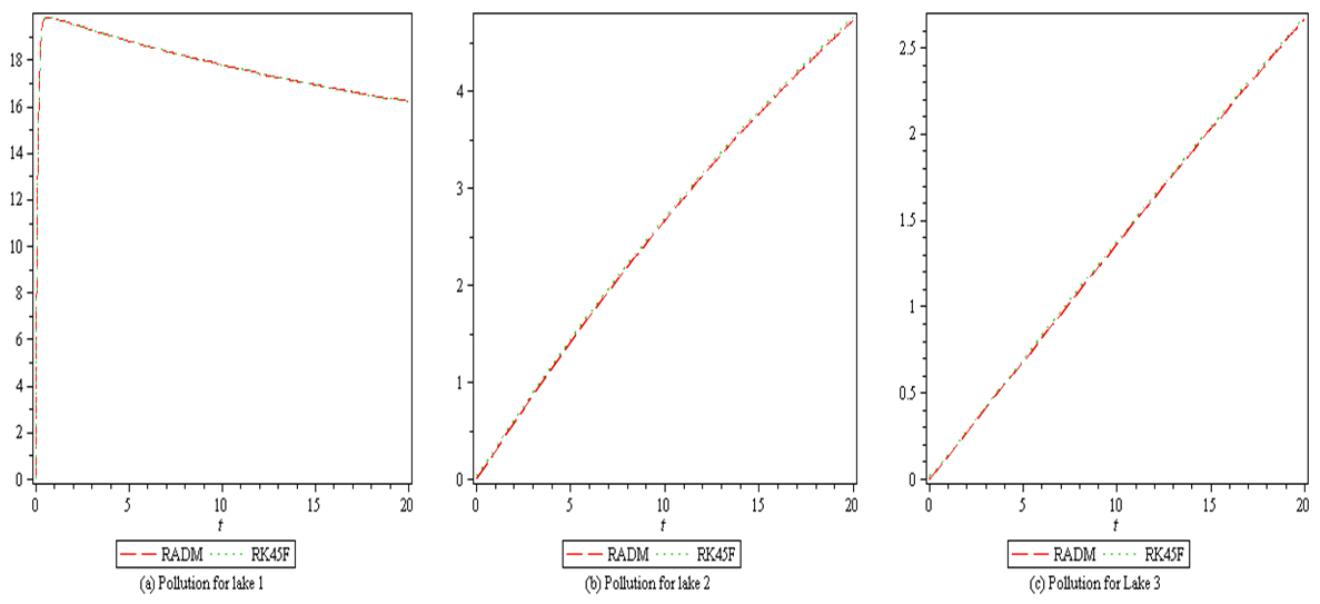Figure 4. Graphical representation of exponentially decaying input pollutant in Lake 1, 2 and 3 with RADM and RK45F solutions. The time is expressed in years

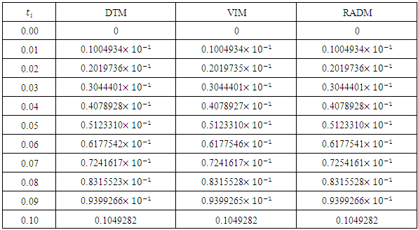
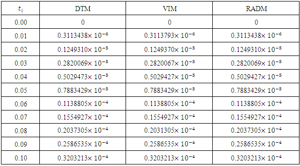
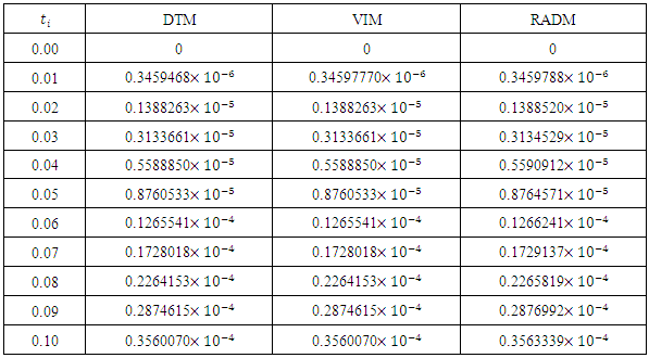
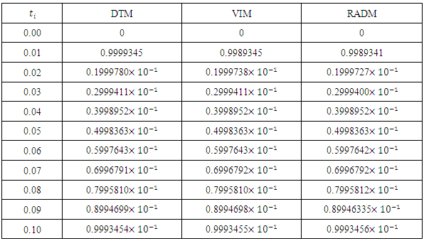
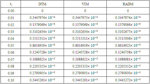
5. Discussion

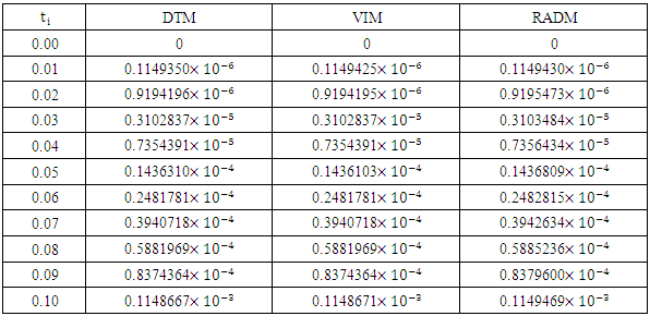
In this paper, we presented the Revised A domain decomposition method (RADM) as a useful semi- analytical technique for solving a pollution model for a system of lakes. Three input models were successfully solved. For each of the three cases solved here, the RADM transformed the dynamic model into a system of Volterra integral equations for the coefficients of the series solutions.

For the purpose of comparison, the Fehlberg fourth order Runge-Kutta method with degree four-fifth interpolant (RK45F) [12-13] built in Maple CAS software was used to obtain the exact of the model. Figure 1, 2 and 3 depicts the comparison among the exact solutions obtained by RK45F method and the RADM approximations for the three input models; sunoisodal, Impulse and step input. We also show in table 1-3, the comparison between the results obtained by the RADM and that of DTM [11] and VIM [7], the results are almost the same. The advantage of the RADM over the both method is that, it converges faster and does not generate secular terms like the VIM.

Other semi-analytical methods like PIA, VIM, HPM and RVIM, among others require an initial approximation for the solutions sought and the computation of one or several adjustment parameters. If the initial approximation is properly chosen, the result obtained can be highly accurate. Nevertheless, no general methods are available to choose such initial approximation. This issue led to the use of Adomian polynomials [2] to solve such nonlinear problems.

On the other hand, RADM just like DTM or LPDTM does not require any perturbation parameter or initial iteration for starting the iteration process. The solution procedure does not involve unnecessary computation and it converges faster to the exact solution of the pollution model. The approximation was made possible and easier using Maple 13.

6. Conclusions

The problem of pollutions of three lakes with interconnecting channels has been considered. Different input models have been used for monitoring the pollution in three lakes. The Revised Adomian decomposition method has been used to solve the solution of the system of linear differential equations governing the problem. The results are compared with those obtained by VIM [7] and DTM [11]. This comparison shows that the results are almost the same, but the solution procedure does not generate secular (noise) terms as the case of VIM, and converges faster to the exact solutions obtained by RK45F method.

ACKNOWLEDGEMENTS

The Authors are grateful to Dr. T. Aboiyar of the University of Agriculture, Makurdi. Nigeria for his useful comments which have improved the quality of this work. We also sincerely appreciates Jafar Biazar of the University of Guilan for the light we have received in some of his publications. Thank you.

Appendix

Table 1a. Comparison between RADM and other methods for pollutant in Lake 1 (sunoisodal input)

Table 1b. Comparison between RADM and other methods for pollutant in Lake 2 (sunoisodal input)

Table 1c. Comparison between RADM and other methods for pollutant in Lake 3 (sunoisodal input)

Table 2a. Comparison between RADM and other methods for pollutant in Lake 1 (Impulse input)

Table 2b. Comparison between RADM and other methods for pollutant in Lake 2 (Impulse input)

Table 2c. Comparison between RADM and other methods for pollutant in Lake 3 (Impulse input)

Table 3a. Comparison between RADM and other methods for pollutant in Lake 1 (Step input)

Table 3b. Comparison between RADM and other methods for pollutant in Lake 2 (Step input)

Table 3c. Comparison between RADM and other methods for pollutant in Lake 3 (Step input)