1. Introduction

The nonlinear response of a suspended elastic cable under random excitation at 2:1 internal resonance of the first planar and non-planar modes is investigated. The Gaussian and non-Gaussian closure solutions are found to be in a good agreement with Monte-Carlo simulation. It is indicated that the mean response of the in-plane mode possesses a non-zero mean under zero mean excitation due to the non-zero sag-to-span ratio [1]. A three-mode, first in-plane mode and first two out-of-plane modes, random excitation of a suspended elastic cable with a 2:1:2 internal resonance is considered and studied. The Fokker-Planck equation and non-Gaussian closure scheme are applied to perform random analysis, which are validated using Monte Carlo simulation. The effect of some cable parameters on the autoparametric interaction is investigated [2]. The nonlinear dynamics of a two d.o.f. suspended elastic cable under small tangential oscillations of one support, which result in parametric excitation of out-of-plane motion and simultaneous parametric and external excitation of in-plane motion, are studied. A first order perturbation analysis is applied to determine the stability of the planar and non-planar periodic motions and found that suspended cables may exhibit saturation and jump phenomena. Theoretical predictions are found to be in a good agreement with experimental measurements of the cable two-to-one resonant response [3]. A second order perturbation analysis is conducted to investigate the existence and stability of periodic solutions with near commensurable natural frequencies in a two-to-one ratio. It is found that cubic nonlinearities disrupt saturation and theoretical results are confirmed by numerical integration of the equations of motion [4]. A three degree-of-freedom model of suspended elastic cable subject to planar excitation is considered and the resonant response of the system is studied when a symmetric in-plane mode interacts with two out-of-plane modes. The considered simultaneous internal resonance occurs when the natural frequency of the in-plane mode is in the neighborhood of natural frequency of the first out-of-plane mode and of twice of natural frequency of the second out-of-plane mode. The multiple scales method up to a second order is utilized to obtain periodic solutions, which are verified numerically [5]. The case of 1:1 internal resonance and primary parametric resonance of a two dimensional suspended elastic cable to parametrical excitation of out-of-plane motion and external excitations of in-plane motion is studied. The theory of normal form and method of multiple scales are used to obtain a simplified averaged equations. It is shown that the considered model may undergo Hopf bifurcation, heteroclinic bifurcations and a Silnikov type homoclinic orbit to the saddle focus. Numerical simulations are performed to illustrate the theoretical predictions [6]. A hyprid three-dimensional finite element/incremental harmonic balance method is utilized to study the nonlinear modal interaction and internal resonance of a suspended cable. It is found that response profiles of the cable at the super-harmonic resonance are very different from those at the primary and internal resonances. Moreover, strong modal interaction occurs in the transition from the primary resonance to the super-harmonic resonance, and from the superharmonic resonance to the primary resonance [7]. The nonlinear responses of immersed cable subject to constant fluid flow speed along the cable plane with two in-plane mode interaction under fluid hydrodynamic forces are investigated. It is indicated that the system exhibits a periodic attractor in the configuration plane when the velocity of the fluid is large [8]. The non-planar finite dynamics of a four d.o.f. elastic suspended cable to external excitations and support motions are studied. The equations of motion, which represent two in-plane and two out-of-plane components, are solved using the method of multiple scales of order two considering the cases of primary external resonance and three simultaneous internal resonances. The effect of some control parameters is investigated [9]. The case of three-to-one internal resonance between the modes of the beam and the string in the presence of subharmonic resonance for the beam is considered and examined. The method of multiple scales is applied to study the steady-state response and the stability of the model. The effect of different parameters on the system is studied and several nonlinear behaviors of the system are found, which are confirmed numerically [10]. The dynamics of cable with concentrated loads were investigated using a direct perturbation method combined with multiple time scales. The model was assumed to have complex loads, including nonlinear aerodynamic force and concentrated masses [11]. The dynamic configuration of inextensible cables was studied [12]. Three components of displacement describing two equilibria of an extensible, traveling, elastic cable were obtained [13]. Simple formulas were established to analyze the global vibration of a cable-stayed bridge [14]. The global bifurcations of an inclined cable under external excitation with external damping are studied and the case of primary resonance is considered. The Shilinkov type homoclinic orbits and chaotic dynamics are analyzed using a new global perturbation technique [15]. The nonlinear dynamic responses of cable structures with two-to-one internal resonance cases [16-18], and three-to-one internal resonance [19] are studied using different methods and the chaotic dynamics of the cable model is illustrated by numerical simulations. Primary and subharmonic resonance cases in an inclined cable under external harmonic excitation are investigated theoretically and experimentally [20].

The present work examines the nonlinear resonant behavior of one in-plane mode that is coupled with two out-of-plane modes. The Galerkin method is used to discretize the governing nonlinear equation of motion into three ordinary differential equations with quadratic and cubic nonlinearities. Using the method of multiple scales, a set of first order nonlinear differential equations are obtained. The analytical results show that the system behavior includes several characteristics of the nonlinear system in the resonant frequency response curves. It is also shown that the system parameters have various effects on the nonlinear response of the considered model.

2. Cable Model Formulation

The elastic cable of length L suspended between two supported ends, one is fixed and the second is vibrating support is shown in Fig. 1. The external excitation is assumed to be harmonic loading of the form f₂(s)cosΩt acting upon the elastic cable in the tangential (in-plane) direction of the cable’s left support.

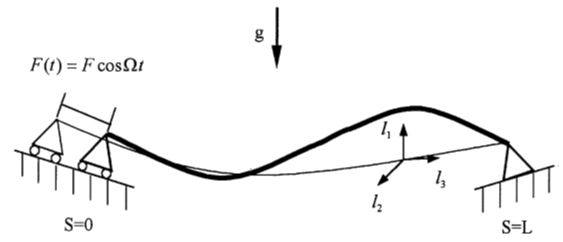Figure 1. Schematic diagram of the suspended elastic cable, [6]

The model of the considered cable under investigation is very close to the one studied by Perkins [5]. The nondimensional equations governing the transverse motion of a suspended is given by:

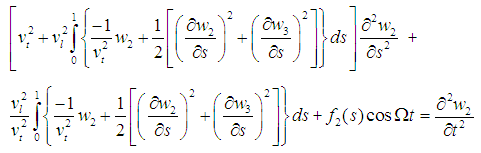(1)

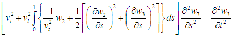(2)

associated with the following boundary conditions for k = 2,3. are nondimensional displacements with respect to the static equilibrium configuration of the cable in the normal and binormal directions, respectively, s is the nondimensional arc length coordinate of the cable and t is the nondiemnsional time. and denote the nondimensional transverse and longitudinal wave speeds of the cable, respectively.

The partial differential equations (1) and (2) are discretized considering one in-plane mode and two out-of plane modes using the following expansions, which represent separable solutions

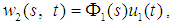(3)

(4)

where is the in-plane mode shape with the corresponding natural frequency ω₁ and are out-of-plane mode shapes with the corresponding natural frequencies ω_1,2. These mode shape functions are obtained by substituting Eqs. (3) and (4) into the linear equations of motion governing the free motion about the equilibrium position for normal and binormal directions, that are extracted from Eqs. (1) and (2). Then using separation of variables and applying the boundary conditions gives:

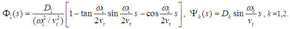where D₁ and D_k are arbitrary constants. Substituting Eqs. (3) and (4) into Eqs. (1) and (2), applying the applying the Galerkin method and adding linear viscous damping coefficients µ_1,2,3 lead to the following three nonlinear coupled ordinary differential equations in terms of the nondimensional generalized coordinates u_1,2,3(t):

(5)

(6)

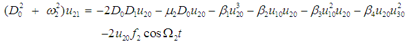
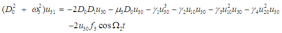
(7)

where

u₁, and u_2,3 are the displacements of in-plane and out-of-plane modes of the cable, associated with natural frequencies ω₁, and ω_2,3 and viscous damping coefficients µ₁, and µ_2,3, respectively, α_i for i=1…6, β_j and γ_j for j = 1…4 are nonlinear parameters, is a small perturbation parameter, F and Ω₁ are the in-plane external forcing amplitude and frequencies, f_j ( j =1,2,3) and Ω₂ are parametric forcing amplitudes and frequency. These parameters are defined as follows

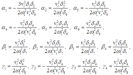where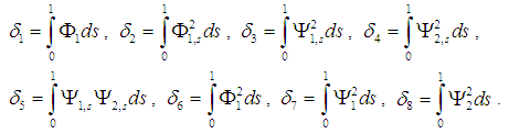

3. Perturbation Analysis

A generalization of the method of multiple scales [21] is utilized to obtain a first-order uniform expansion for the solutions of Eqs. (5-7) in the form.

(8)

where, .

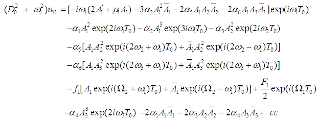
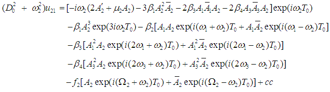
Substituting Eq. (8) into Eqs. (5-7) and equating the coefficients of the same powers of ε , yield the followingOrder ε⁰:

(9)

Order ε1:

(10)

(11)

(12)

The solutions of Eq. (9) can be written in the following form

(13)

where cc denotes the complex conjugate of the preceding terms. By substituting Eq. (13) into Eqs. (10-12), we obtain the following equations:

(14)

(15)

(16)

where the prime indicates the derivative with respect to T₁.

The general solutions of Eqs. (14-16) can be expressed in the following forms:

(17)

(18)

(19)

where A_1,2,3 are complex functions in T₁, which are still arbitrary at this level of approximation. They can be determined by eliminating the secular terms at the next approximation.

We consider the simultaneous resonance conditions which occur when the primary parametric resonance conditions Ω₂ ≈ 2ω₁ ≈ 2ω₂ ≈ 2ω₃ are satisfied simultaneously between three modes of vibration, which mean the existence of the primary internal resonance ω₁= ω₂= ω₃. Furthermore, primary parametric resonances of in-plane and out-of-plane modes lead to primary external resonance of the in-plane mode (Ω₁ ≈ ω₁), where for convenience of the investigation we assume Ω₂ = 2Ω₁. The closeness of the resonances is described by

(20)

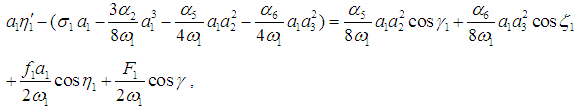
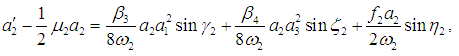
where σ, and σ₁, σ₂, σ₃ denote primary and parametric external detuning parameters, respectively. The definitions (20) are used in Eqs. (14-16) together with the polar representation , k = 1,2,3, and the eliminating of the secular terms provides the following four equations governing the amplitude and phase modulations

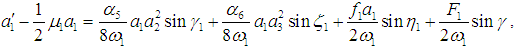(21)

(22)

(23)

(24)

(25)

(26)

where

γ = σ T₁ – θ, γ₁ = 2(θ₂ – θ₁), ζ₁ = 2(θ₃ – θ₁), η₁ = σ₁ T₁ – θ₁, γ₂ = 2(θ₁ – θ₂), ζ₂ = 2(θ₃ – θ₂), η₂ = σ₂ T₁ – θ₂, γ₃ = 2(θ₁ – θ₃), ζ₃ = 2(θ₂ – θ₃), η₃ = σ₃ T₁ – θ_3.

The steady-state periodic responses of the three modes of vibrations correspond to constant solutions, that is correspond to and , for j = 1,2,3. Using these conditions in Eqs. (21-26) leads to

(27)

(28)

(29)

(30)

(31)

(32)

The above Eqs. (27-32) have the following possible solutions:

(1) pure in-plane motion (a₁ ≠ 0, a₂ = a₃ = 0),

(2) pure out-of-plane motion (a₁ = 0, a₂ ≠ 0, a₃ ≠ 0)

(3) primary and parametric resonant motion (a₁ ≠ 0, a₂ ≠ 0, a₃ = 0), (a₁ ≠ 0, a₂ = 0, a₃ ≠ 0), and (a₁ ≠ 0, a₂ ≠ 0, a₃ ≠ 0), which is the practical case.

We shall consider and study the last case (a₁ ≠ 0, a₂ ≠ 0, a₃ ≠ 0), which is the practical one among the previous mentioned cases. The frequency response equations of this case are given by:

(33)

(34)

(35)

4. Numerical Results

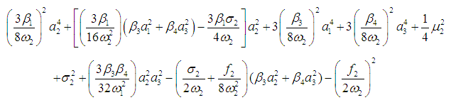
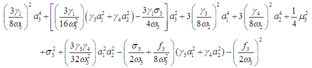
The steady-state periodic solutions corresponding to the fixed points of Eqs. (27-32) for simultaneous internal and principle parametric resonances of the three modes are obtained when the conditions are implemented. From the resulting equations, the frequency response Eqs. (33-35) are obtained and solved numerically using the MAPLE^© software.

The analysis of local stability is determined by linearization of Eqs. (21-26) for the parameters a₁,_2,3 and η_1,2,3 about each singular point, which will result in a set of linear equations with constant coefficients and hence lead to an eigen-value problem. Then, these eigen-values associated with the resulting linear equations will be examined. If the real part of every eigen-value of the coefficient matrix is positive then the point is unstable, otherwise must be stable. These linear equations are formed by assuming that each one of the parameters a₁,_2,3 and η_1,2,3 is expressed in the form

(36)

where a_n0 and η_n0 are the solutions of the steady-state Eqs. (21-26) when and and a_n1 and η_n1 are small perturbations. Inserting Eq. (36) into Eqs. (21-26) and keeping the linear terms in a_n1 and η_n1, then solving the resulted the state-space equation , where the matrix [A] is the Jacobian matrix, in order to calculate the eigen-values.

The numerical results are presented in Figs. (2-5) as the steady-state amplitudes a_1,2,3 are varied against the detuning parameters σ_1,2,3 for different values of the system parameters. In these figures, Each curve consists of right and left branches. The left branch stands for the stable solutions and the right one stands for the unstable solutions.

Considering Fig. (2a) as a basic case for comparison, where σ₁ is plotted against a₁ (in-plane mode). It can be seen from Figs. (2b) that as the linear viscous damping coefficient µ₁ increases, the steady state amplitude of the first mode a₁ decreases. Figures (2c) and (2d) show several representative curves for the cubic nonlinear term α₂. Comparing these curves shows that the nonlinearity effect (either hardening or softening nonlinearity) bends the frequency response curves to right when α₂ is positive and to left when α₂ is negative. The figures also illustrate the variation of the steady-state amplitude as α₂ is varied. The remaining cubic nonlinear terms α₅ and α₆, Figs. (2e, 2f), do not strongly change the amplitude as they are varied and hence no effect on the response curves. As the natural frequency ω₁ increases, Fig. (2g), the branches of the response curves converge, and the region of unstable solutions decreases. The steady-state amplitude a₁ is increased as the parametric excitation amplitude f₁ increases as shown in Fig. (2h), whereas Fig. (2k) indicates that the variation of the external forcing amplitude F₁ shows different effect and behavior on the frequency response curves. In Figs. (2i) and (2j), the resonant response curves are shifted to right as the steady-state amplitudes of the second and third modes a₂ and a₃ are increased.

In addition, the force response curves presented in Fig. 3 illustrate the variations of the steady-state amplitude a₁ with the forcing parametric excitation f₁ for different values of the cubic nonlinear terms α₂, α₅ and α₆. The significant effects of α₅ and α₆ are shown in Figs. (3c) and (3d), where the first mode amplitude increases as these nonlinear terms increase.

For the second mode of vibration (first out-of-plane mode), the steady-state amplitude a₂ is plotted against the detuning parameter σ₂, as shown in Fig. (4). These curves illustrate the effects of the damping coefficient µ₂, the cubic nonlinear terms β_1,3,4, the natural frequency ω₂, the parametric excitation amplitude f₂, the steady-state amplitudes of the first and third modes a₁ and a₃.

The force response curves of the second mode of vibration for different values of the damping term and nonlinear terms are shown in Fig. (5). It is noticed from Fig. (5b) that as the parametric excitation amplitude f₂ increases beyond 25.0, the effect of increasing the linear damping coefficient µ₂ becomes insignificant and the steady-state amplitude a₂ of the first out-of-plane mode saturates. It is also noted that the curves are shifted to the right as µ₂ is increased further, which means that the amplitude of the excitation f₂ must exceed a critical value before the first out-of-plane amplitude a₂ is to be strongly excited.

Similar effects and curves are reported for the variation of the second out-of-plane amplitude a₃ with σ₁ and f₃ for different values of system parameters, therefore they are not included in the figures.

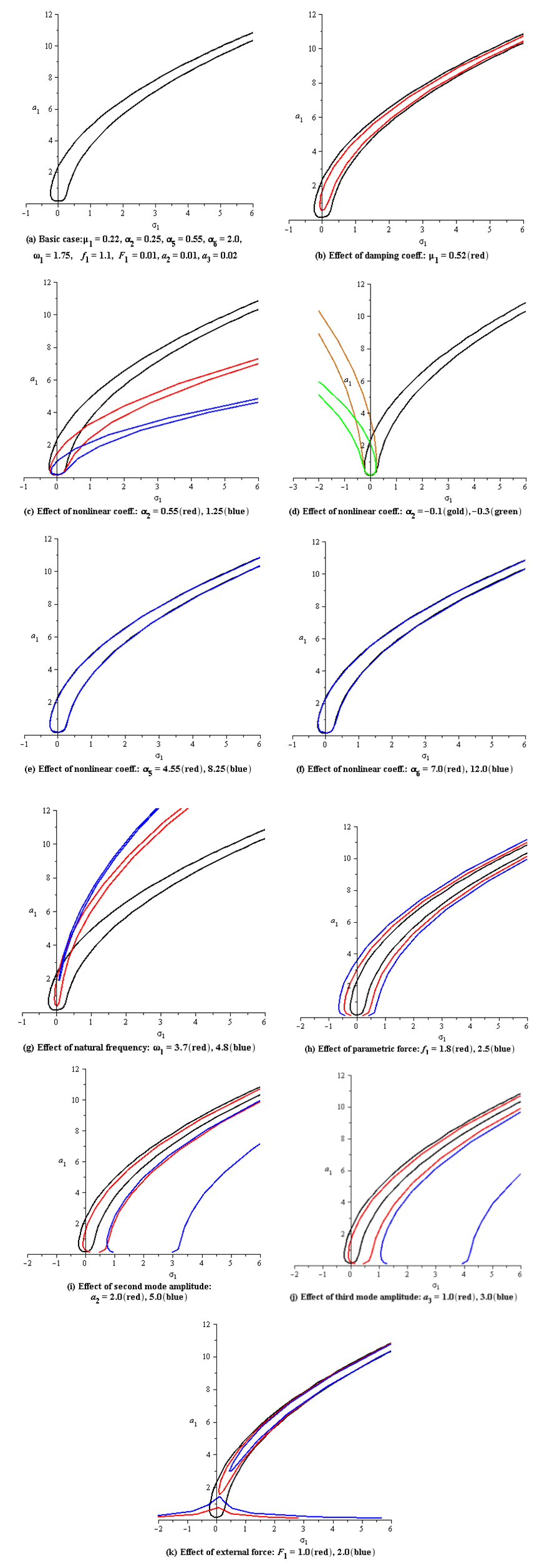Figure 2. Resonant frequency response curves for the first mode of the system

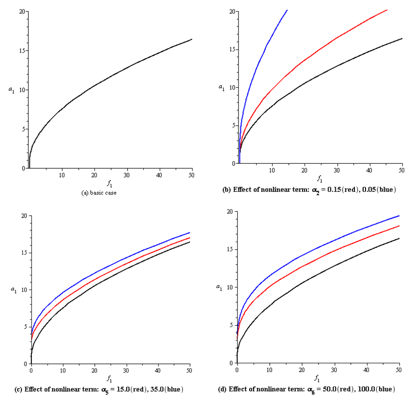Figure 3. Resonant force response curves for the first mode of the system

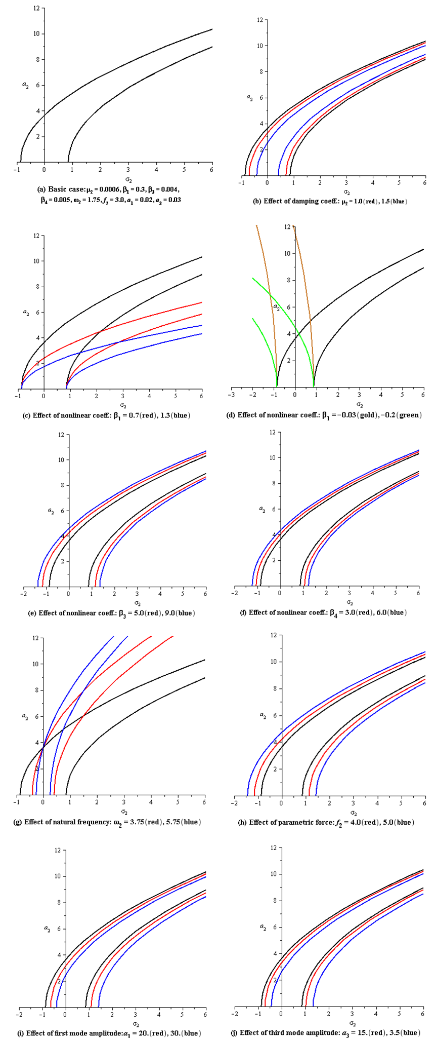Figure 4. Resonant frequency response curves for the second mode of the system

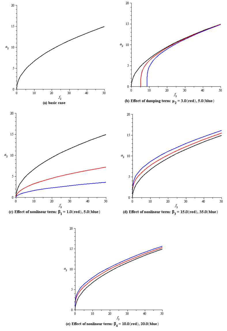Figure 5. Resonant force response curves for the second mode of the system

5. Conclusions

The nonlinear response of an elastic suspended cable to small tangential vibration of one support has been studied. The problem is described by a three-degree-of-freedom system of nonlinear ordinary differential equations, which represent one in-plane equation and two out-of-plane equations. The case of 1:1:1 internal resonance in the presence of principal parametric resonance between the in-plane and out-of-plane modes is studied by applying a perturbation method using a first-order approximation. The frequency response equation is numerically solved to obtain the steady-state solutions and to investigate the effects of different parameters on the system behavior.