Ognjen Vukovic
Department for Finance (MSc student), University of Liechtenstein, Liechtenstein
Correspondence to: Ognjen Vukovic, Department for Finance (MSc student), University of Liechtenstein, Liechtenstein.
| Email: |  |
Copyright © 2015 Scientific & Academic Publishing. All Rights Reserved.
Abstract
Author of this paper tries to apply Heisenberg Uncertainty Principle in time series analysis. After implementing the Heisenberg Uncertainty principle and making a connection between quantum mechanics and time-series analysis, notion of Gabor atom has been introduced. Gabor atom is a concept also taken from quantum physics and it is characterized by the minimal time-spread in time frequency plane. After developing the theory characteristic to Gabor atom, it was shown that the original time series can be reconstructed from Gabor’s resonance coefficient by using double integral. At the same time, it is proved that there is no problem with the time-frequency localization of Gabor frames at the critical density. It is shown that from a practical point of view the issue of time-frequency concentration still exist, but only in the form of numerical instabilities or bad condition numbers for critically sampled Gabor frames.
Keywords:
Gabor atom, Heisenberg Uncertainty Principle, Time series analysis, Quantum physics, Risk management, Asset pricing, Fourier transform, Compact groups
Cite this paper: Ognjen Vukovic, Heisenberg Uncertainty Principle and Gabor Atom in Time-Series Analysis, Applied Mathematics, Vol. 5 No. 3, 2015, pp. 73-76. doi: 10.5923/j.am.20150503.03.
1. Introduction
When considering uncertainty, the following concept must be applied:Schroeder said that one of the fundamental consequences of uncertainty is the very size of atoms, which, without it, would collapse to an infinitesimal point. [1]. Uncertainty is defined as lack of certainty, not being able to make a decision on a safe basis.In order to approach Heisenberg uncertainty principle, firstly we must define Heisenberg uncertainty principle in quantum mechanics. Uncertainty principle is defined as any variety of mathematical equations that provide limited knowledge of certain pairs of physical properties of complementary variables that can be known pertaining in that sense to complementary variables like position  and momentum
  [1].The uncertainty principle states the main characteristic of quantum systems.
2. Theoretical Background
Heisenberg principle applied in risk management and time-series analysis can be formulated in the following way [2]:The Uncertainty principle asserts that there are no time series with finite risk which is compactly supported both in the time and frequency domains [2].In order to prove the following assertion, we will compare two approaches. One approach is classical quantum approach, where we will try to establish analogy between quantum physics and time series analysis and the other one is classical econometrical approach [3].Firstly, we will demonstrate classical econometrical approach taken from Cornelis Los [2].We define equivalent time duration  of
of  by
by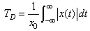 | (1) |
where  At the same time, we define the spectral bandwidth
  of
of  by
by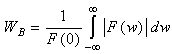 | (2) |
where  Uncertainty principle by Heisenberg states that the product of equivalent spectral bandwidth and time duration of a time series
  cannot be less than a certain minimum value, which is given by the following equation.
 | (3) |
The proof is the following: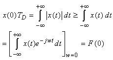 | (4) |
Similarly, if we do the same for  we have
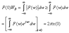 | (5) |
Using these two equations, we obtain the following: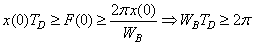 | (6) |
The conclusion is that Uncertainty principle in time-series analysis holds and the following equation proves it: | (7) |
If we want to compare it to Heisenberg principle of uncertainty in quantum physics, we use the equation given by Earle Hesse Kennard and Herman Weyl. | (8) |
where  represents the standard deviation of momentum while
  denotes the standard deviation of position of a particle.The two equations look very similar, except that here Plack constant plays its role because of quantum phenomenon.In order to continue our analysis, we will repeat the uncertainty principle which states that there is no finite risk time series
  which is supported in time and frequency domains. In other words, according to Cornelis A. Los [2] the risk spread of variable and Fourier time-frequency cannot be simultaneously small. In order to surmount the aforementioned problem, we will take idea from Hungarian physicist Gabor who defined, inspired by quantum physics, elementary time-frequency ‘atoms’ or ‘kernels’ that have minimal time-spread in the time-frequency plane.Gabor atoms [4] are given by the following form and are constructed by time translation by period
  and frequency modulation (frequency
  ) of the original time window
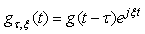 | (9) |
such that 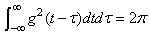 | (10) |
Gabor’s atom [4] is a product of sinusoidal wave  with a finite risk symmetric window. The risk of
  is dependable and simmetrically concentrated in the time neighborhood of
  over an interval size
  measured by the standard deviation of
  and with a frequency center
  Gabor atoms can be seen as changing analyzing filters which adapt to frequency in time series
  associated with frequency
  in the neighborhood of time horizon
  The Fourier transform of the Gabor atom is a frequency translation by
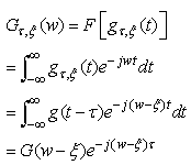 | (11) |
The equation above proves that the risk of  is localised near the frequency
  over an interval of size
  so it measures the domain where Gabor resonance coefficient
  is non-negligible.How can this be applied to time-series analysis?The original Fourier transform[5] represents a time series as the sum of sinusoidal waves in which resonance coefficients are correlation coefficients. The aforementioned sinusoidal waves are because of Uncertainty principle, very well localized in frequency, but not in time, since their support has infinite length. But we want to analyse time series that are very well localized both in time and freqency something that is similar to Gabor atoms.If we take for example Heisenberg box. Gabor’s Heisenberg Box is centered at
  and has a time dispersion
  and a frequency dispersion
  . The Uncertainty principle proves that Heisenberg box satisfies the following inequality:
 | (12) |
What the following inequality proves is that there cannot exist an instantaneous frequency analysis for finite risk time series. Therefore time-frequency localization is achievable only in the mean squares sense as visualized by Heisenberg box. To be more thorough we can say that if the time series  is non-zero with compact support, then its Fourier transform in the frequency domain cannot be zero on a whole frequency interval. At the same time, if Fourier transform is compactly supported, then the time series cannot be zero on a whole time interval.So the definition or better axiom is the following:If the Heisenberg constraint is satisfied, it is impossible to have a function in
  space, which is compactly supported both in time and frequency domain.In order to finalize, we will show how original time series
  can be reconstructed from Gabor’s resonance coefficients by the following double integral.Firstly, we represent Gabor’s Transform as a scalar function, with two arguments, time horizon
  and frequency
  Gabor’s Transform correlates the time series
  with each Gabor atom
  to produce the following resonance coefficients:
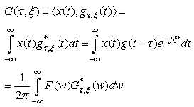 | (13) |
The last equation is a consequence of Parseval’s Formula: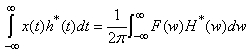 | (14) |
If we put in Parseval’s formula  we obtain:
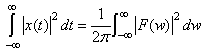 | (15) |
again using Parseval’s formula.As a final result, we would like to present a formula demonstrating the reconstruction of original time series  from Gabor’s resonance coefficient by the following double integral. The formula is the following:
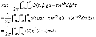 | (16) |
The above given equation represents a time series as a sum of localized waves weighted by the profile of the chosen taper or window. This shows that Gabor’s Transform has a constant time-frequency resolution. This resolution can be changed by rescaling the window  This is easy to model and represents the complete, stable and redundant representation of the systematic part of time series.In order to conclude, we will introduce a spectrogram which can be used to measure the risk of financial time series
  in the time frequency neighborhood of
  that is given by the Heisenberg box. This implies that it is possible to measure and visualize the localized risk of a financial time series, instead of average risk.The formula is given below:
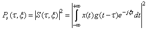 | (17) |
where  is a spectral line
 is a windowed Fourier resonance coefficient
 is a frequency that depend on the time
3. Theoretical Results
The results we obtained are based on the following Heisenberg hypothesis:If the Heisenberg constraint is satisfied, it is impossible to have a function in  space, which is compactly supported both in time and frequency domain.It is known that on
  Gabor frames at the critical density are not an appropriate tool for time –frequency analysis. The proof of that is based on Balian-Low theorem [6].Balian-Low theorem states the following:If a Gabor system
 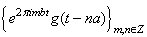 with
with  forms an orthonormal basis for
 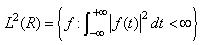 then
then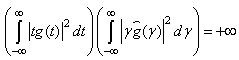 | (18) |
where 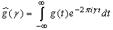 is the Fourier transform of
  is the real line and
  is the set of integers.The Balian-Low theorem proved the square-integrability of the partial derivatives of the function, but it didn’t imply continuity of the function itself in two dimensions and higher.As with the Uncertainty principle this formulation cannot be extended to arbitrary local compact abelian groups because of lack of differentiation operators and lack of canonical weights.However we will be considering groups containing compact open subgroup.Proposition. If
  is a local compact abelian group containing a compact open subgroup K, then there exist a window
  and a discrete set
  such that
 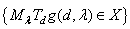 is an orthonormal basis for
  and
and 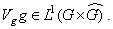 Proof of the aforementioned proposition can be found in Grochenig paper [6].Whereas on R the short Fourier transform is obviously not in
  , and the corresponding (orthonormal basis) ONB is badly localized in frequency, it is really interesting to see the window
  constructed on
  We will want to show that the Fourier transform of compact open subgroup is in the Fourier algebra.We have the following:
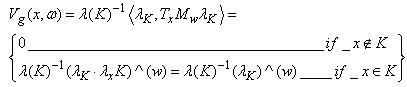 | (19) |
So we get the following: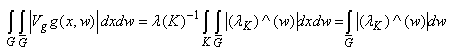 | (20) |
Since we have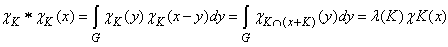 | (21) |
the following result is obtained: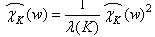 | (22) |
If we integrate both sides, the following is obtained: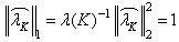 | (23) |
This proved that  This result proved that in discrete and compact groups which are used for numerical simulation- there is no problem with the time frequency localization of Gabor frames at the critical density [6].
4. Conclusions
This paper presented a novel approach to time-series analysis by using tools of quantum physics. Quantum finance is a slowly developing subject, but this paper made a little contribution to its development. It introduced Heisenberg Uncertainty Principle in time series analysis and at the same time introduced the notion of Gabor atom which enabled the reconstruction of original time series. It proved that Heisenberg Uncertainty principle in time- series analysis can be surmounted by using Gabor atom by proving that discrete and compact groups which are used for numerical simulation exhibit no problem with the time frequency localization of Gabor frames at the critical density. The given approach is interesting and has further application in time series analysis.
References
| [1] | Busch, P., Heinonen, T., & Lahti, P. (2007). Heisenberg's uncertainty principle. Physics Reports, 452(6), 155-176. |
| [2] | Los, C. (2006). Financial market risk: measurement and analysis. Routledge. |
| [3] | Los, C. A. (2001). Computational finance: a scientific perspective. World scientific. |
| [4] | Shi, Y., & Zhang, X. D. (2001). A Gabor atom network for signal classification with application in radar target recognition. Signal Processing, IEEE Transactions on, 49(12), 2994-3004. |
| [5] | Bracewell, R. (1965). The Fourier Transform and IIS Applications. New York. |
| [6] | Feichtinger, H. G., & Strohmer, T. (Eds.). (2012). Gabor analysis and algorithms: Theory and applications. Springer Science & Business Media. |
 Abstract
 Reference
 Full-Text PDF
 Full-text HTML